Introduction
This online manual provides a single, authoritative reference for all Rhopoint Instruments hardware and software, supporting users from initial setup through to advanced application and data reporting. It is designed for operators, quality and laboratory personnel, R&D teams, and system integrators using Rhopoint solutions in both production and laboratory environments.
About Rhopoint Instruments
Rhopoint Instruments is a UK-based manufacturer of quality control test equipment, specialising in the measurement of surface and material appearance. The portfolio has evolved from glossmeters to include instruments for gloss, haze, DOI, texture, defect analysis, shade, opacity, transparency, coefficient of friction, and packaging performance.
Responsibilities and prerequisites
This manual assumes that users are familiar with basic laboratory and production safety procedures, and that instruments are operated within the environmental and electrical conditions specified in each product section. It does not replace site-specific risk assessments or quality system documentation; rather, it is intended to be integrated into existing ISO-based quality frameworks and local operating procedures.
Instruments and Hardware
Instruments
Rhopoint Aesthetix
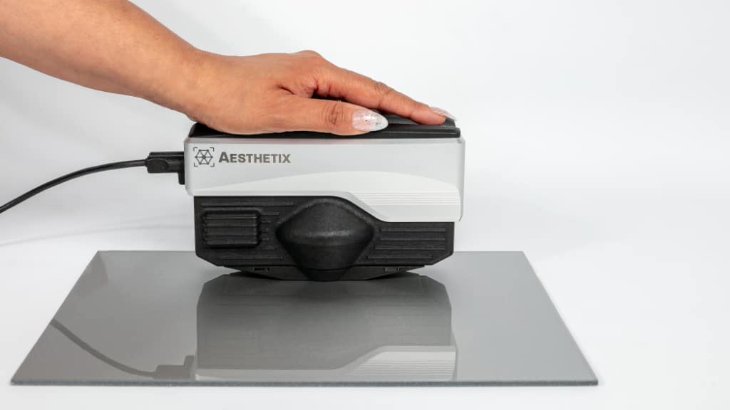
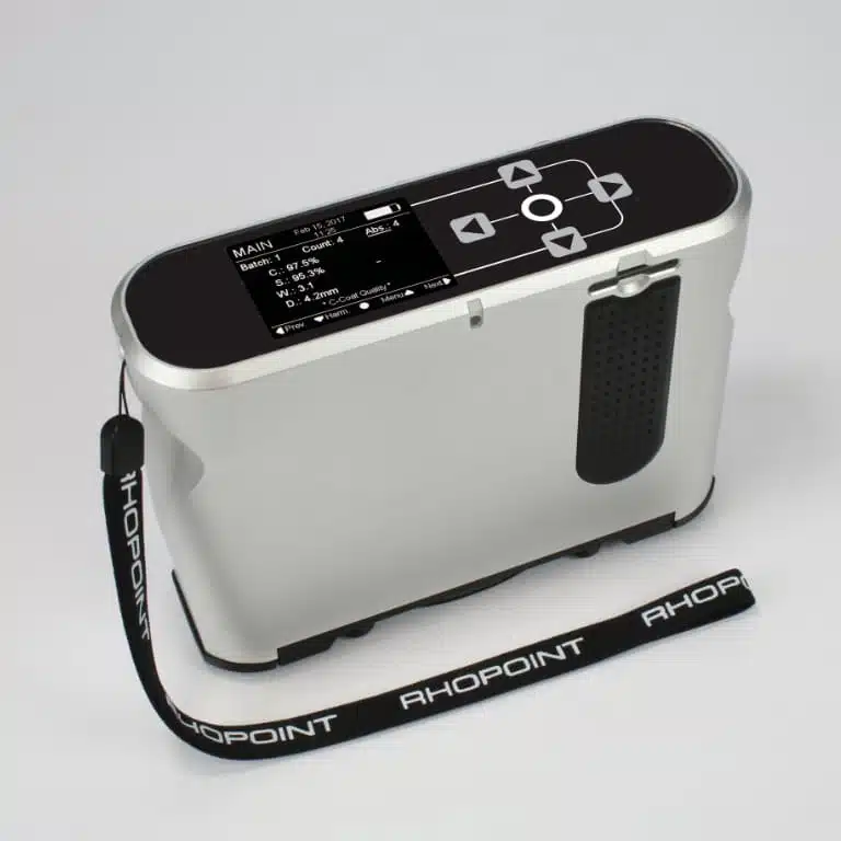
Rhopoint Aesthetix is a modular dual camera‑based sensor that captures detailed images of a surface under controlled lighting to assess gloss, haze, texture, sparkle, waviness and defects. It connects to a Windows PC over USB and utilises perception based metrics to reports how surfaces will look to the human eye. Rhopoint Aesthetix
Rhopoint TAMS
Rhopoint TAMS is a hand‑held instrument for high end, high gloss surfaces, evaluating how good a finish looks overall and how well parts match each other. A low gloss module also checks E‑coat, plastic and similar raw materials, describing surface roughness and waviness making it possible to link early process steps to final appearance. Rhopoint TAMS
Rhopoint Aesthetix
What is Rhopoint Aesthetix?
Rhopoint Aesthetix is a modular, camera‑based surface appearance sensor that measures how real surfaces look to the human eye across a wide range of materials, including paints, plastics, metals and textured coatings. It uses high‑resolution imaging, controlled multi‑angle illumination and interchangeable adaptors to capture detailed reflection and surface images from flat panels, small parts and curved components in both laboratory and production environments.
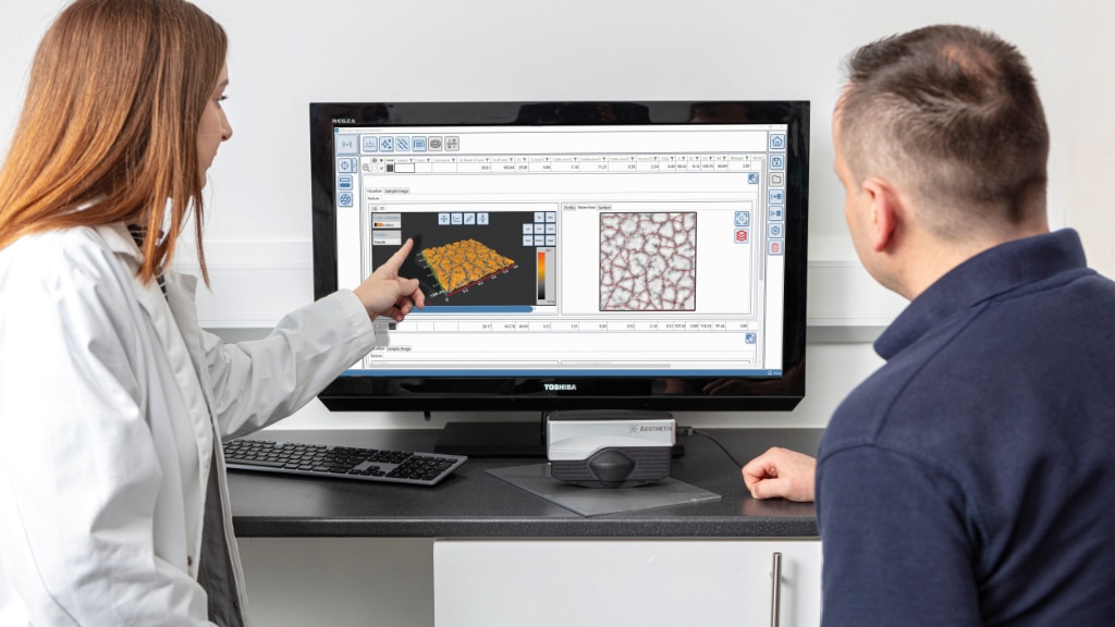
In a single measurement, Aesthetix can characterise multiple aspects of appearance—such as texture, waviness, haze, DOI, sparkle, graininess, scratches and other visible defects—and link each metric directly to stored images. This image‑driven approach makes it easier for operators, quality engineers and R&D teams to define visual targets, compare materials and processes on a common scale, and communicate appearance requirements clearly across the organisation.
Getting Started
The Aesthetix is a camera-based measurement sensor that is not a stand‑alone instrument and must always be used in combination with Rhopoint Appearance Elements or Elemants Hub software. This page explains the basic setup requirements and how to connect the sensor so it can be safely and correctly controlled by the software.
System requirements
Aesthetix must be connected to a compatible Windows 11 PC or tablet with Rhopoint Appearance Elements or Rhopoint Headless Elements installed; it cannot perform measurements or display results on its own. The host device must have an available USB 3.0 port, sufficient storage for images and results, and user permissions to install and run the software.
Software
The Rhopoint Aesthetix can be used with two software packages-
Appearance Elements (AE) is Rhopoint Instruments PC based measurment and data analytics software.
Using Aesthetix with Appearance Elements
Headless Elements (HE) is a headless connection hub for third party applications such as SPC, PLC and laboratory management software.
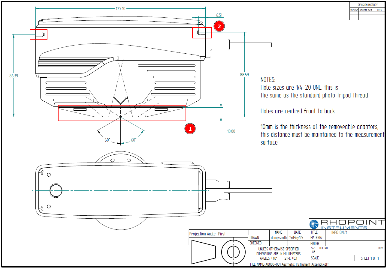
Specifications and Dimensions
| Device | Aesthetix |
|---|---|
| Size (H x L x W) [mm] | 104 x 177 x 83 |
| Weight [g] | 802 |
| Power | USB 3.0 Port on controlling PC/Tablet (7.2W max, 2.4W min) |
| Control | Software triggered measurement or read button on instrument |
| Interface | USB 3.0 USB-C or Thunderbolt |
| Indoor/Outdoor | Portable equipment can be used indoor or outdoor but primarily lab use. |
| Altitude | Up to 2000 meters |
| Temperature | Operating temperature: 15°C - 40°C (60°F - 104°F) |
| Relative humidity | Operating humidity: Up to 85% (non condensing) |
| Specular Optics | |
|---|---|
| Geometry | 60° |
| Measurement spot size [mm] | 9 x 18 ellipse (2 x 4 with adaptor) |
| Aspecular Optics | |
|---|---|
| Geometry | 10°x:0°; 45°c:0°; 60°x:0°; 20mm linelight |
| FOV [mm] | 18 x 24 |
| Analyzed Area [mm] | varies |
| Resolution (surface) | 9.2 µm/pixel (109 pixel/mm) |
Curved Surfaces & Non-Contact Measurement
The Rhopoint Aesthetix sensor uses a modular, magnetic base system that accepts a range of jigs and adapters for different sample types and geometries. These accessories can be quickly removed and reattached, enabling repeatable positioning for flat panels, curved components, small parts and delicate surfaces in both contact and non‑contact configurations.
To remove an adapter, pull gently on it to separate it from the base. The adapter is held in place magnetically, so it will release cleanly without tools when a light, even pulling force is applied.
Standard Adaptor (included with standard Aesthetix)
Flat surfaces- ideal for laboratory measurement of test panels Standard Adaptor
Curved Surface and small area gloss adaptor (included with standard Aesthetix)
Measure gloss in a smaller area and measurement of cylindrical parts. Curved surface and small area gloss adaptor (2mm spot)
Small Parts
Gloss, Haze and DOI measurement of small parts- Novo Curve small aperture adaptor
Improved Grip on Flat Surfaces
Non slip rubber feet improve measurement improve positional stability on high slip surfaces, ideal for in field measurement- Four-point rubber contact adaptor.
Improved Grip on Cylindrical Parts
Non slip rubber feet improve measurement improve positional stability on high slip surfaces, ideal for in field measurement of large cylinders- Four-point rubber contact adaptor.
Improved Grip on Large-radius Complex curved surfaces
Non slip rubber feet improve measurement on high slip surfaces, ideal for in field measurement- Three‑point rubber contact adaptor
Curved Surfaces
Complex Curved Surfaces- Three-point rubber contact adaptor - small aperture
Non-Contact measurement
Small area gloss adaptor (needed for measuring gloss of curved surfaces)- Non-contact measurement
Standard Adaptor (included with standard device)
The standard adaptor is designed for contact measurements on flat, rigid panels and is the default choice for most Aesthetix applications in paints and coatings laboratories. It provides a gloss measurement spot of approximately 9 mm by 12 mm, allowing the instrument to average appearance over a relatively large area that is representative of typical coated test panels and production parts.
The standard adaptor is supplied as standard with the Aesthetix sensor.
Part Number- B8000-031
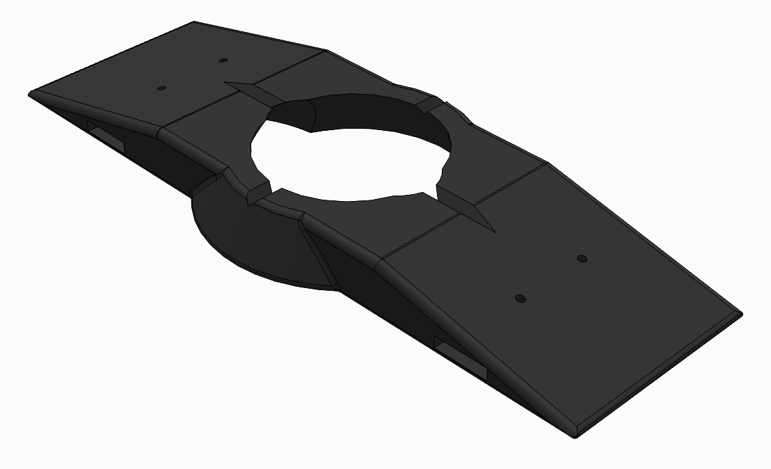
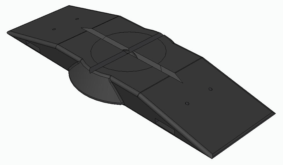
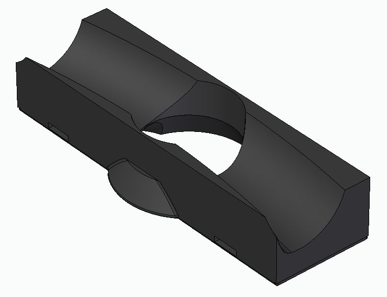
Curved surface and small area gloss adaptor (included with standard device)
Small Area Gloss Adaptor
The small area gloss adapter is designed for curved surfaces or for resolving gloss in small areas where the standard Aesthetix gloss measurement spot is too large. The V-shaped cutouts are designed to allow accurate positioning of small cylindrical components.
It reduces the gloss measurement aperture from 9 × 12 mm to approximately 2 × 3 mm, allowing accurate measurements on tighter curves and small localised areas that need to be individually identified and characterised.
The flat smooth base of this adaptor makes it most suitable for flat panels or very gently curved surfaces.
For more complex curved surfaces consider the three or four point adaptors.
The small area gloss adaptor is supplied as standard with the Aesthetix sensor.
Part Number B8000-032
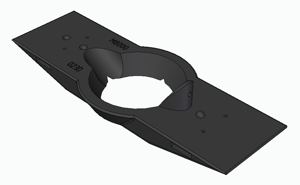
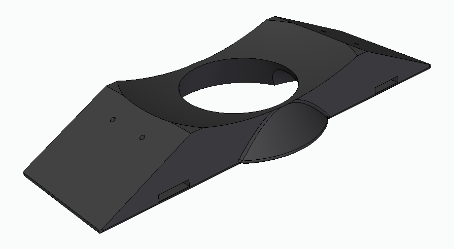
Novo Curve small aperture adaptor
The Novo-Curve small aperture adapter converts the Aesthetix sensor into a Novo-Curve–style glossmeter for very small parts and features. When this adapter is fitted the instrument is used upside down so that small components can be placed and manipulated on top of the adapter surface. The V-shaped cutouts are designed to allow accurate positioning of small cylindrical components.
With this adapter, the measurement port is reduced to a hole of approximately 2-3 mm diameter, allowing precise gloss measurements on tiny areas that are difficult to measure with the standard aperture. Small parts can be manually positioned and rotated during measurement to find and characterise the exact region of interest.
When the Novo-Curve small aperture adapter is attached, the 0° camera path is blocked, so the 0° images and live view are not available. In this configuration the instrument can only be used for standard gloss, haze (without compensation) and DOI measurements and not for full image-based Aesthetix metrics.
Part number- B8000-041
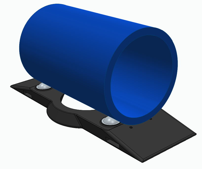
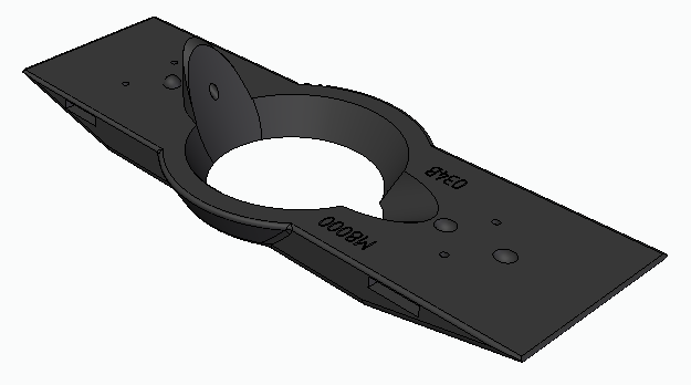
Four-point rubber contact adaptor - small aperture
The four‑point rubber contact adaptor is designed for measuring cylindrical and regularly curved objects such as pipes, tubes and rods. With the 2 mm gloss spot size provided by the small‑area optics, the device is suitable for measuring the gloss of cylinders with diameters down to 40 mm, while still maintaining reliable alignment on the curvature.
Its four certified rubber contact points support the instrument along the long axis of the object, positioning the gloss aperture precisely on the curved surface for stable, repeatable readings. The rubber material is compatible with paint shop environments and minimises the risk of marking fresh or sensitive coatings during measurement.
For best results when measuring cylinders place the instrument along the flattest edge of the sample as shown below.
Part Number B8000-040
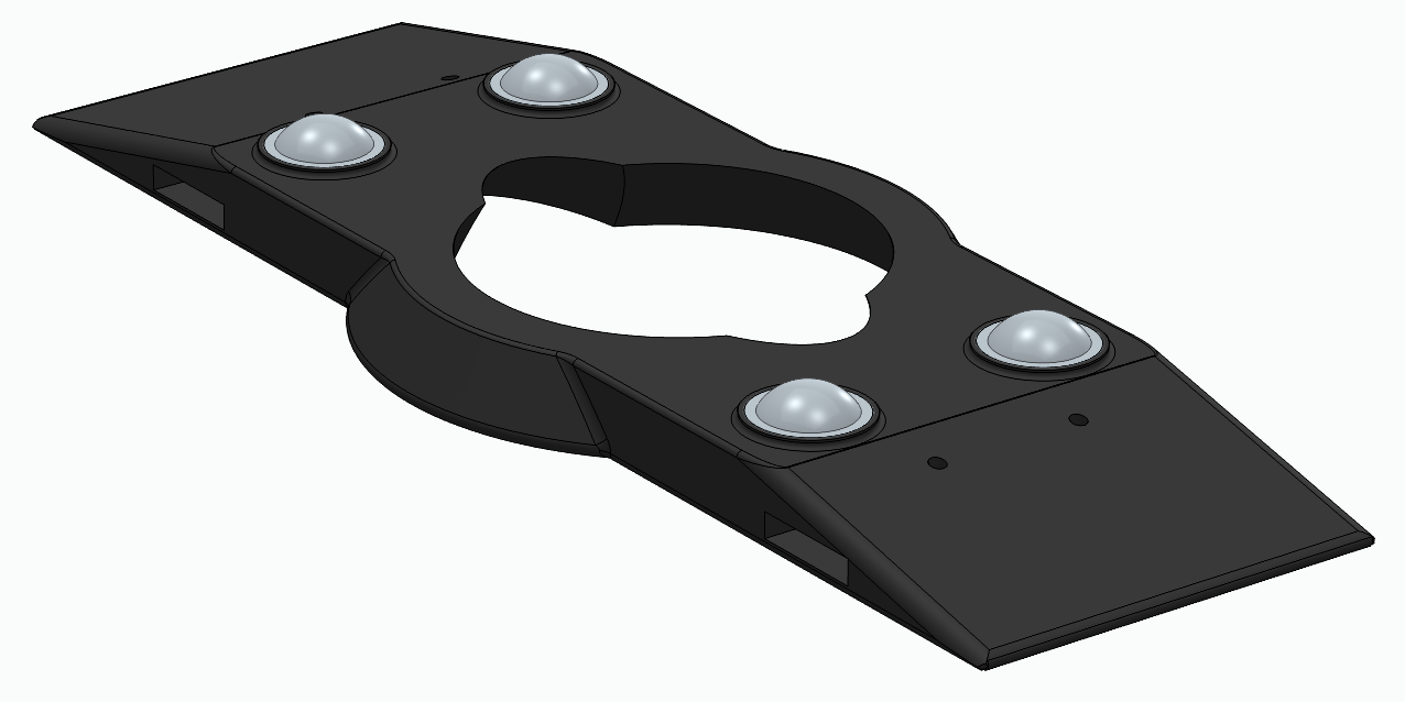
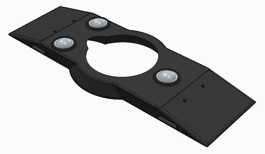
Four-point rubber contact adaptor
The four‑point rubber contact adaptor with the standard gloss aperture is intended for measuring flat panels and other planar surfaces where extra stability is required. It retains the normal Aesthetix gloss spot size, making it suitable for general paints and coatings applications while improving instrument handling on larger samples.
Four certified rubber contact elements support the instrument at the corners of the adaptor, helping the sensor sit flat and securely on the surface during measurement. This added stability reduces the risk of sliding, improving repeatability and making it easier to obtain consistent gloss, haze and DOI readings on panels in laboratory and production environments.
Part Number- B8000-039
Three-point rubber contact adaptor - small aperture
The three‑point rubber contact adaptor with small aperture is designed to improve stability when measuring complex curved surfaces using a tripod contact arrangement. Three rubber feet support the instrument at well‑defined points, helping it sit securely on irregular or multi‑axis curves while keeping the optics correctly oriented to the surface.
This adaptor incorporates the small‑area gloss aperture, enabling accurate measurements on localised features and tight radii where the standard spot size would be too large. The combination of tripod stability and reduced measurement area makes it particularly suitable for small, contoured components and detailed inspection zones on complex geometries.
Part Number- B8000-036
Three‑point rubber contact adaptor
The three‑point rubber contact adaptor with the standard gloss aperture is designed to improve stability when measuring complex curved or slightly irregular surfaces. Three rubber feet form a tripod support, helping the instrument sit securely on the surface and maintain the correct orientation for the standard gloss measurement spot.
Because the standard gloss aperture is retained, this adaptor is suitable for routine gloss, haze and DOI measurements where a full‑size measurement area is required but positioning is more challenging. The tripod contact pattern reduces rocking and variation in contact, improving repeatability on contoured panels and other parts that are not perfectly flat.
Part Number- B8000-035
Bespoke jigs and fixtures
Bespoke Jigs
The Rhopoint Aesthetix can be used with 3D-printed jigs for repeatable measurement of small parts or curved surfaces.
To design your own jigs and fixtures, contact Rhopoint to receive a 3-D design advice pack with example STL’s.
Non-Contact Small Area Gloss Adaptor (2mm)
Non-Contact Measurement
The Non-Contact Small Area Gloss Adaptor (2mm) is designed to allow non-contact measurement when using the Aesthetix with a Lab Stand, Co-Bot or mounted on a custom designed frame/jig. The adaptor must be used with a gap of 2mm between the bottom face and the sample to be measured.
This adaptor incorporates the small‑area gloss aperture, enabling accurate measurements on localised features and curved parts.
Part Number- B8000-034
Adaptor Mount
The adaptor mount is designed to allow multiple mounting options for the Aesthetix, it attaches to the Aesthetix using the mounting holes on each end of the device. It is provided with the lab stand but can also be purchased separately.
Part Number- B8000-300
The adaptor mount has two options for mounting the device, direct mounting on the measurement stand or four mounting holes designed to take M6 socket cap screws.
Central hole is used in the lab stand, 4 remaining holes can be used for mounting using M6 screws.

If using the lab stand attach the adaptor plate to the adaptor mount using the thumb screw.
Attach the mount to the Aesthetix using the supplied 1/4 UNC screws.
Adaptor mount fitted showing the lab stand adaptor plate.
Laboratory Measurement Stand
The Rhopoint Aesthetix Lab Stand enables users to take precise, non‑contact measurements of delicate materials and curved surfaces, ensuring accuracy without risking damage or deformation. Curved parts can be manipulated using live view to ensure correct alignment.
Part Number- B8000-010
Procedure for non-contact measurement
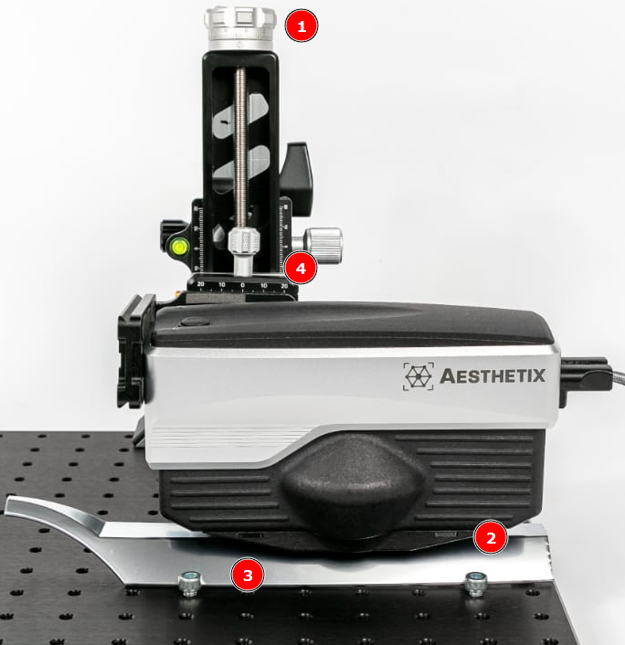
The pre-calibrated Aesthetix should be attached to the stand with the standard or small area gloss adaptor attached.
Set Focal Distance
-Place the part (3) to be measured on the stand.
-Wind the part until the bottom plate is in contact with the measurement surface,
Check positioning
-Use the interactive measurement mode to ensure the correct part of the sample is in the FOV, and if measuring gloss that the gloss reflection is in the middle of the sensor. How to measure Surface Brilliance
-Note the height of the laboratory stand z-axis (4)
Remove Base
-Lift the Aesthetix (1) and remove the base, if measuring the gloss of curved parts replace with the non-contact small area gloss adaptor.
-Wind (1) to the correct height (4) z-axis (4)
-Use the interactive measurement mode to check the correct part of the sample is in position, and that the gloss reflection is in the middle of the sensor. How to measure Surface Brilliance
-Measure the sample.
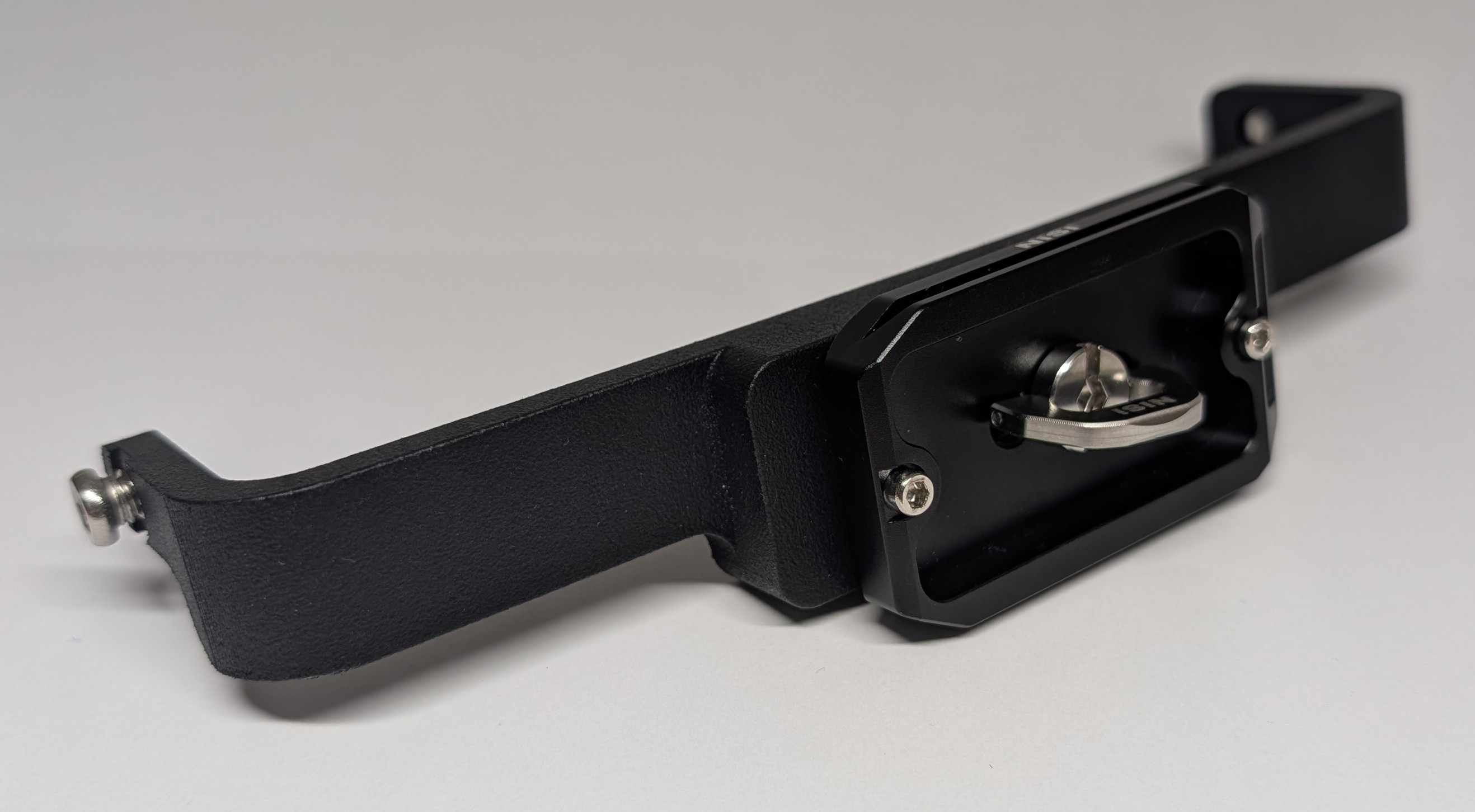
Cobot and Inline Setup
Fixing the Aesthetix
The Aesthetix aluminium chassis should be fixed at two points (2)
Rhopoint supply fixtures and brackets that can be used to integrate to Cobot/Robot or inline mounting points - contact us for more details.
Positioning the device- contact measurement
Before taking a measurement the device must be positioned so that the base of the adaptor is in contact with the surface and completely flat.
Procedure for non-contact measurement
If measuring the gloss of curved parts the non-contact small area gloss adaptor should be attached.
-For all other measurments the bottom adaptor (1) should be removed.
-Position the sensor sensor so the bottom part of the Aesthetix (without base) is 10mm from the surface.
-Use the interactive measurement mode to check the correct part of the sample is in positioned in the FOV, and that the gloss reflection is in the middle of the sensor. How to measure Surface Brilliance
Considerations for Non-contact measurement
Ambient lighting- measurments are largely unaffected by changes in ambient light conditions, however do not use outside or in direct sunlight without shielding optics from gross changes in light conditions.
Positional Accuracy- For accurate measurement the focal distance must be maintained to 10mm +/- 0.2mm (measured from the bottom of the sensor unit) with a maximum angular error of +/- 0.5° parallel and perpendiular to the measurement plane
Moving Material- Gloss, Haze, DOI measurements can be measured on a moving line, other measurements which require observer camera images require a stationary material.
Cleaning the Aesthetix
Cleaning the Aesthetix sensor
This page explains how to clean the Aesthetix sensor optics and contact surfaces to maintain reliable measurements while avoiding damage to the instrument or samples.
Safety and general rules
- Do not attempt to open the sensor housing.
- Always stop measurements in the software before cleaning.
- Never use household cleaners, abrasive materials or unapproved solvents on any part of the sensor or adaptors.
Cleaning the sensor lenses and optical window
The optical window and internal lenses are precision components and must only be cleaned using a dedicated lens cleaning kit (e.g. camera/optical lens kit including blower, lens brush and lens tissues or cloth).
- Inspect the window under good lighting for dust, fingerprints or smears.
- Use the blower from the lens kit to remove loose dust; do not use your breath.
- If particles remain, use the soft lens brush from the kit with very light strokes.
- For fingerprints or smears, apply a small amount of lens cleaning fluid to a lens tissue/microfiber from the kit (never directly to the window).
- Wipe the window gently in straight lines, then dry immediately with a fresh lens tissue.
Do not:
- Use paper towels, standard cloths or cotton buds.
- Press hard, scrub in circles or reuse dirty tissues.
- Spray or drip liquid directly onto the sensor.
Cleaning adaptors and contact surfaces
- Remove the adaptor from the sensor.
- Wipe the outer contact faces and rubber feet with a clean, lint‑free cloth slightly dampened with water or mild detergent if required; then dry thoroughly.
- Keep the measurement opening free from paint, dust and fibres; if needed, use the blower from the lens kit around the aperture (avoiding direct contact with the optics).
Avoid solvents that could attack rubber or plastic parts, and ensure all surfaces are completely dry before re‑attaching the adaptor.
Good practice to prevent contamination
- Store the sensor and adaptors in their case when not in use.
- Avoid placing the instrument face‑down on dusty or painted surfaces.
- Do not measure on uncured or heavily contaminated coatings.
Storage and Handling
Storage and handling
To maintain performance, the Aesthetix should be stored and handled as a precision optical instrument.
- Avoid impacts: Do not knock, drop or subject the instrument to shock as this may damage optics or electronics.
- Temperature stabilisation: If the instrument has experienced a large temperature change, allow it to stabilise to ambient before use to prevent internal misting.
- Environmental protection: Prevent exposure to moisture, chemicals and corrosive vapours during storage and operation.
- Measuring aperture: Do not insert objects into the measuring aperture; this can damage the measuring system.
- Cleaning: Clean housing and screen only with a soft, slightly moist cloth; chemical resistance cannot be guaranteed for all solvents.
- Sunlight and humidity: Avoid prolonged direct sunlight, continuous high humidity or condensation.
Packing List
Package contents
Aesthetix sensor with USB-C connector
Gloss module calibration standard
USB stick containing:
- Appearance Elements software installer
Lanyard hand strap
Small part and curved surface adapter
Calibration certificates
Printed quick start guide
Cleaning Cloth
Optional:
- Texture measurement calibration standard
- Rubber base standard adapter
- Rubber base small part and curved surface adapter
- Measurement stand
- Non-contact small part and curved surface adapter
- Bespoke part adaptors
- USB-A connector cable
- 3m connector USB-C cable
Rhopoint TAMS
What is Rhopoint TAMS?
Rhopoint TAMS (Total Appearance Measurement System) is a portable, imaging‑based instrument that quantifies how reflective surfaces actually appear to a human observer. It was developed with Volkswagen AG for automotive body panels, but the same principles apply to any product where perceived finish quality is critical, including domestic appliances, consumer electronics, plastic components, decorative metalwork and coil‑coated sheet.
TAMS uses Phase Measurement Deflectometry and high‑resolution surface mapping to capture how a surface reflects and distorts structured patterns in less than 10 seconds, directly on the part. The instrument generates detailed 2D and 3D data and converts this into perception‑based High Gloss metrics such as Contrast, Sharpness, Waviness and Dimension, along with composite indices Quality (Q) and Harmony (H) that describe overall appearance and panel‑to‑panel matching in a way that aligns with human vision.
In separate a Low Gloss mode, TAMS focuses on surface topography and roughness for stages such as raw material, E‑coat and primer. The full‑field altitude map is filtered using ISO GPS‑style methods (for example ISO 16610 / ISO 25178 concepts) to generate optical roughness and waviness values compatible with modern surface specifications, linking roughness control directly to final visual appearance.
High Gloss Mode
High Gloss Mode overview
High Gloss Mode evaluates smooth, reflective surfaces where visual impression is critical, such as painted panels, plastics, decorative metals, glass and high‑gloss coatings. TAMS projects a series of patterns onto the surface and uses techniques such as Phase Measurement Deflectometry, Optical Transfer Function analysis and line deformation methods to characterise how the surface reflects and distorts these patterns. This behaviour is condensed into a set of perception‑based metrics, so users can see at a glance how good a finish looks and how closely different parts or samples match.
Quality and Harmony metrics
High Gloss Mode reports two main indices: Quality (Q) and Harmony (H).
- Quality (Q) describes the overall visual appearance of a high gloss surface, combining contrast, sharpness and waviness into a single 0–100% value, where 0% indicates a poor, dull or highly distorted finish and 100% represents a mirror‑like surface.
- Harmony (H) describes how similar two high gloss surfaces are when viewed side by side, for example adjacent panels or reference versus production. A value below 1 suggests that most observers would accept the difference in texture and orange peel between the two; values above 1 indicate differences that many viewers are likely to notice and find unacceptable.
These indices are designed to follow how people actually judge surfaces, making them suitable for specification, process control and communication with non‑specialists.
Colour‑dependent perception in High Gloss Mode
TAMS Quality automatically includes basecoat colour through the contrast parameter, so dark and light colours are handled correctly. Contrast depends on colour—white and metallic finishes have low contrast, while deep black can approach 100%—which changes how strongly texture, haze and DOI are seen.
Because colour is built into the measurement, surfaces with very different colours can be controlled on the same Quality and Harmony scale, instead of using separate limits or rules for each colour shade. This simplifies specifications and ensures that appearance control reflects what people actually see on the finished product.
Underlying appearance parameters
To calculate Quality and Harmony, TAMS first extracts several sub‑characteristics from the reflected image.
- Contrast (C) measures the difference between bright highlights and dark areas in the reflection and is directly linked to surface colour: deep black, high‑impact finishes give high contrast, while white and metallic surfaces have low contrast.
- Sharpness (S) quantifies how clearly details are reflected. At close distances it indicates how well fine features are reproduced; at normal viewing distance it is closely related to haze and clarity. Values range from 0% (blurred, low definition) to 100% (very crisp reflection).
- Waviness (W) describes the overall wave‑like distortion of the reflection caused by larger‑scale texture or orange peel. A value of 0 corresponds to a visually flat surface with minimal distortion; values up to around 30 represent increasingly wavy, distorted reflections.
- Dimension (D) indicates the dominant texture scale seen at a typical viewing distance of around 1.5 m. It is expressed in millimetres, typically between 0.5 and 8 mm, and helps distinguish fine, tight texture from coarse, large‑scale structure.
Together, these parameters allow High Gloss Mode to summarise complex reflection behaviour into intuitive numbers that match visual perception and support both quality control and process optimisation on any high gloss surface.
Low Gloss Mode
Low Gloss Mode is used to evaluate surfaces where texture and roughness dominate the visual impression, such as pre‑treated metals, primers, electro‑coats, matt and semi‑gloss finishes, and many raw or semi‑finished materials. In these situations, the final appearance of any high‑gloss topcoat depends strongly on the underlying roughness and waviness, so measuring earlier process steps provides valuable insight and control.
In this mode, TAMS generates a full‑field 3D altitude map of the surface and derives roughness‑ and texture‑based parameters from this map.
Quality Control roughness and texture parameters
Low Gloss Mode reports several key indices from the altitude map, without applying additional filtering in the standard algorithm.
- Optical‑Ra (O‑Ra) is an image‑based equivalent of the familiar Ra parameter, calculated as the arithmetical mean deviation of the altitude profile across the measured area. It is derived from the 3D map, so it captures roughness over a defined field rather than a single line.
- Optical‑Rq (O‑Rq) is the root‑mean‑square deviation of the altitude profile, analogous to Rq in classical roughness analysis. Like O‑Ra, it is computed from the full‑field elevation data to give a robust description of surface height variation.
- Waviness describes the larger‑scale movement of the surface texture using slope information and standard deviation calculations. Values run from 0 (very low texture) to around 30 (very strong texture), and are often influenced by upstream processes such as rolling, forming or blasting.
- Quality (Q) in this mode is derived from waviness and expressed on a 0–100 scale, providing a single indicator of how smooth or textured the surface is from a process standpoint.
These parameters allow users to quantify how well different stages (for example substrate, pre‑treatment, low gloss coatings) prepare a surface for later finishing, and to understand which processes have the greatest impact on final appearance.
Advanced roughness analysis
For applications that require more classical ISO‑style roughness evaluation, Low Gloss Mode can be extended with the O‑Rough algorithm. In this configuration, TAMS applies ISO‑16610 band filtering to the altitude map before calculating roughness characteristics.
Users can define high‑pass, low‑pass or band‑pass filters, including multiple bands, to isolate specific wavelength ranges of interest. After filtering, TAMS calculates parameters such as Sa, RaX, RaY and RsM according to ISO 25178, using the full measurement field. This provides a direct bridge between TAMS measurements and traditional profilometers or areal topography systems, making it easier to compare results, set shared limits and integrate low gloss surface control into existing ISO GPS‑based specifications.
Getting Started with TAMS
System requirements
TAMS can be used as a hand‑held, stand‑alone instrument, operated directly via its built‑in screen, menus and on‑board storage for fast checks on the line, in the lab or at the audit station.
When you want PC control and advanced analysis, TAMS can be connected to a compatible Windows 10 or 11 PC or tablet with Rhopoint software installed. The host device should provide a stable USB connection (or approved wireless link), sufficient storage for maps and results, and user permissions to install and run Rhopoint applications.
Software
TAMS works with two Rhopoint software platforms:
- Appearance Elements (AE) – full GUI software for running measurements, viewing TAMS maps and images, and managing jobs, batches and reports alongside other Rhopoint instruments.
- Headless Elements (HE) – a background service used when TAMS is integrated into automated or third‑party systems, providing measurement control and data access without the full AE user interface.
Calibrate the TAMS
Calibrate the TAMS
Before taking measurements, calibrate TAMS using the supplied plate so focus and reference values are correctly calibrated.
Calibration plate
The plate includes three tiles:
- Plastic‑ref – for surface focus.
- Silver‑ref – for screen focus and reference calibration.
- Check tile‑ref – for later verification only (not used during calibration).
Start calibration
- On the instrument, select Menu → Calibration → Start calibration process.
- Confirm with YES and press OK.
Step 1 – Plastic‑ref
- Place TAMS on the Plastic‑ref tile (top tile).
- Ensure all four feet are flat on the tile.
- Select Continue and press OK.ly calibrated
TAMS now sets the surface autofocus.
Step 2 – Silver‑ref
- Move TAMS to the Silver‑ref tile (mirror‑like middle tile).
- Ensure all four feet are flat on the tile.
- Select Continue and press OK.
TAMS now sets the screen autofocus and reference calibration, then returns to normal operation.
Step 2 – Gloss
- Move TAMS to the Gloss‑ref tile.
- Ensure all four feet are flat on the tile.
- Select Continue and press OK.
TAMS now calibrates the gloss measurement.
Select Surface Type and Algorithim
High Gloss Mode – select surface type and algorithm
To use High Gloss Mode, TAMS must be set to the correct surface type and algorithm so that Quality and Harmony are calculated for smooth, reflective finishes.
Choose the High Gloss surface type
- Open the Menu.
- Go to My Car (or the surface settings section, depending on firmware).
- Set Surface type to the option used for high‑gloss, top‑coated surfaces (typically C‑Coat or equivalent in your version).
This tells TAMS that measurements will be taken on smooth, reflective finishes rather than low‑gloss or raw surfaces.
Select the High Gloss algorithm
- Open Menu → Admin → Quality control algorithm.
- For the chosen surface type (for example C‑Coat), scroll through the available algorithms.
- Select the standard High Gloss algorithm (typically CC‑TAMS‑STD or the site‑specific High Gloss mode name).
- Confirm the selection with OK.
In this configuration, TAMS reports the sub‑parameters Contrast (C), Sharpness (S), Waviness (W) and Dimension (D) for each measurement, and uses them to calculate the perception‑based indices Quality (Q) and Harmony (H) after batching.
When to use other algorithms
If special evaluation methods are required for particular products or customers, additional High Gloss algorithms may be available as options under the same surface type. These can be selected in the same way as CC‑TAMS‑STD. Custom algorithms should only be used where specified by internal procedures or Rhopoint support; otherwise the standard High Gloss mode is recommended for general use.
Take a measurement
Measure with TAMS
This section explains how to take a basic measurement with TAMS and how to interpret the status LED during the measurement cycle.
Before measuring
- Ensure TAMS has been calibrated on the supplied plate.
- Check that the aperture and the surface are clean and dry.
- Select the correct surface type and algorithm (for example High Gloss or Low Gloss) in the menu.
Start a measurement
The current shutter mode is shown by the letter in the centre button on the main screen:
- M – Manual: Press the middle touch key or the lower side button to start a reading.
- S – Sensor: Lower TAMS onto the surface; when sensor mode is active, contact on the feet automatically starts the measurement.
- A – Auto: Press the middle key once to start an automatic sequence of measurements.
Keep the instrument still once the measurement has been triggered.
LED status during measurement
The LED near the aperture shows the measurement status and when it is safe to move TAMS:
- Red LED – TAMS is capturing images and 3D height data. Keep the instrument firmly in place with all four feet on the surface; do not move it.
- Blue LED – Image capture is complete and TAMS is calculating results. It is now safe to lift or move the instrument away from the surface.
- Green LED – The measurement cycle is finished and results are available on the main screen for review.
View the results
After the LED turns green:
- The main screen displays the key parameters for the active mode (for example Contrast, Sharpness, Waviness, Dimension, Quality, Harmony, O‑Ra or O‑Rq).
- Batch name, result index and job mode are shown in the header and footer.
- Use the left/right keys to scroll through stored results, and the Info key to see configuration and job details linked to the measurement.
All measurements are saved automatically in TAMS and can be reviewed on the instrument or exported via SD card for further analysis.
Batching Measurements
Batching measurements with TAMS
Batching is used to group several individual measurements on the same part, surface or condition and to calculate averaged values such as Quality and Harmony. Working with batches improves repeatability and makes it easier to compare results between samples, lines or process settings.
Why use batches?
- Reduces the influence of local variation or single outliers.
- Provides average values for key metrics (for example Q, H, O‑Ra, O‑Rq, W).
- Organises results by part, panel, process step or job.
For most applications, at least three measurements per batch are recommended.
Batch modes
Batch behaviour is configured in the Admin → Batch settings menu:
- Manual batch mode – The operator decides when to close a batch.
- Auto batch mode – TAMS automatically closes a batch after a set number of measurements (Auto batch count).
Choose manual mode for ad‑hoc measurements and investigations; use auto mode for routine checks where the same number of positions is measured each time.
Creating a batch (manual mode)
- Ensure the correct surface type and algorithm are selected.
- Take a series of measurements on the same part or condition (for example three or more spots on a panel).
- When finished, press and hold the batch button (as defined in your firmware) to close the batch.
- TAMS calculates the average values for that batch and, in high‑gloss mode, adds the Quality (Q) and Harmony (H) indices.
If Job mode is set to Manual or Guided with a database loaded, TAMS can also prompt for a batch name linked to part or job information.
Creating a batch (auto mode)
- In Batch settings, set Batch mode = Auto and choose an Auto batch count (for example 3).
- Take measurements as normal.
- After the specified number of measurements is reached, TAMS automatically closes the batch and calculates the averages and Q/H or roughness indices.
Auto mode is especially useful in guided workflows where the same pattern of points is measured on each part.
Reviewing batched results
On the Main screen, TAMS offers two review modes:
- By result – scrolls through every individual measurement in order.
- By batch (Q&H mode) – jumps between batch averages only (COUNT #0), which include Quality and Harmony in high‑gloss mode.
Use the left/right keys to move through results, and the Info screen to see batch index, count and any job/part information. Batched data can later be exported via SD card and analysed in Smart Manager, Appearance Elements or other tools.
Setting up the batch and job database
Setting up the batching database
The batching database works together with Job Mode to attach part and process information to batches and, in Guided mode, to step through a defined list of parts in a fixed order. It is stored as one or two CSV files loaded into TAMS from the SD card.
Create the main database file (TAMSdatabase.csv)
The main database is an Excel/CSV file with up to 15 columns and up to 100 rows (including the header).
- File name:
TAMSdatabase.csv - Separator: Comma or semicolon (detected automatically).
Structure:
- Column 1 – Part name (required):
List of batch/part names (for example “Panel A”, “Door LH”, “Cover 1”). This name can be used as the batch name and is shown on the main screen in Manual and Guided Job Modes. - Columns 2–15 – Additional fields (optional):
May include model, colour, process step, environment, coating type, repair status, customer, etc.
Up to 15 fields in total (including Part name), with a maximum of 60 characters per entry.
Example:
| Part name | Model | Colour | Process | Environment | Clear coat | Repair |
|---|---|---|---|---|---|---|
| Hood | A123 | Blue | Line 1 | Lab | Type X | None |
| Door | A123 | Blue | Line 1 | Production | Type X | Stage 1 |
| Roof | A123 | White | Line 2 | Exterior | Type Y | Stage 2 |
Fields shown on the Info screen
Up to four database fields can be displayed on the Info screen:
- These must be in columns 2 to 5 of
TAMSdatabase.csv. - Typical choices include model, colour, process and environment, helping identify each batch during review.
Loading the batching database
- Copy
TAMSdatabase.csvto the root of the SD card (not inside a folder). - Insert the SD card into the TAMS SD slot.
- On the instrument, open Menu → My Car → Load database from SD card.
- Wait for the “Loading database completed” message, then return to the main screen.
Job Mode can now use the part list and fields when naming and organising batches.
Using the database with Job Mode
Job Mode is set in Menu → My Car → Job mode and defines how the database is used.
OFF
- Database is ignored.
- Batches are recorded without names; suitable for quick checks.
Manual
- Database is used as a pick‑list when closing batches.
- After a batch is closed, the instrument prompts to assign a name or leave it unset.
- Available names come from Column 1 (Part name) in
TAMSdatabase.csv.
Guided
- Database is used to guide the operator through a predefined list of parts.
- After selecting Start new job/car, identification fields are set, and the next part to measure is shown at the bottom of the main screen.
- Parts are presented in the order they appear in Column 1, or in a sequence list if configured (see below).
In both Manual and Guided modes, part names and associated fields are stored with each batch for easier filtering and analysis later.
Configuring sequence lists (optional)
Sequence lists allow Guided Job Mode to follow different measurement orders (for example S1, S2, S3…) using an additional sequence file.
Step 1 – Add a SEQUENCE field to TAMSdatabase.csv
In TAMSdatabase.csv:
- Add a column named exactly
SEQUENCE(it must not be Column 1). - For each part, enter the sequence ID to which it belongs (for example S1, S2, S3…).
Example:
| Part name | Model | Colour | Process | SEQUENCE | Clear coat | Repair |
|---|---|---|---|---|---|---|
| Hood | A123 | Blue | Line 1 | S1 | Type X | None |
| Door | A123 | Blue | Line 1 | S1 | Type X | Stage 1 |
| Roof | A123 | White | Line 2 | S2 | Type Y | Stage 2 |
Include an entry such as none in the SEQUENCE column for parts that should follow the default order and not use a special sequence.
Step 2 – Create the sequence file (TAMSsequence.csv)
Create a second CSV file:
- File name:
TAMSsequence.csv - Same basic limits as the main database (up to 15 fields, up to 99 items per list).
Structure:
- Each column header is a sequence ID (S1, S2, S3, etc.).
- Under each header, list the Part name entries in the exact order you want them measured in that sequence.
Example:
| S1 | S2 |
|---|---|
| Hood | Roof front |
| Door | Roof back |
| Roof | Trunk |
Save the file and copy it to the root of the SD card alongside TAMSdatabase.csv.
Step 3 – Load and use sequences in Guided Job Mode
- Load both
TAMSdatabase.csvandTAMSsequence.csvfrom the SD card using Load database from SD card. - Set Job mode = Guided in the My Car menu.
- When starting a new guided job, select the desired sequence (for example S1, S2…).
- TAMS will now propose parts in the order defined in
TAMSsequence.csvfor that sequence.
If the sequence file or selected list is not found, TAMS automatically falls back to using the order in Column 1 of TAMSdatabase.csv.
Using the Job Mode
Using Job Mode
Job Mode controls how TAMS organises measurements into named jobs or parts. It can be used simply to record a few readings, or to guide an operator through a predefined list of parts using a database.
Job Mode options
Job Mode has three settings:
OFF
- No job or part information is used.
- TAMS records measurements and batches, but does not ask for batch names.
- Best for quick checks and ad‑hoc measurements.
Manual
- The operator chooses job/part information when closing a batch.
- TAMS can prompt for a batch name taken from a database (for example a list of parts).
- Suitable when parts are measured in flexible order, but still need to be labelled.
Guided
- TAMS guides the operator through a predefined list of parts or positions.
- Each batch is linked to a specific item in the database (for example “Panel A”, “Panel B”).
- Best when a complete product must be measured in a specific sequence.
Set Job Mode in Menu → My Car → Job mode (names may vary slightly with firmware).
Using Manual Job Mode
Manual mode links batches to names, without enforcing a fixed sequence.
- Set Job mode = Manual in the My Car menu.
- (Optional) Load a measurement database from SD card so that part names are available.
- Take measurements and close batches as usual (manual or auto batching).
- When a batch is closed, TAMS prompts whether to assign a name.
- Choose a name from the list (for example a part or job ID) or skip naming.
On the main screen, the current job mode is shown at the bottom (for example “Job mode: Manual”) and the selected batch name appears on the top line.
Using Guided Job Mode
Using Guided Job Mode
Guided mode is designed for repeated, structured measurement routines.
- Set Job mode = Guided in the My Car menu.
- Choose Start new job/car (wording depends on firmware).
- Enter any required identification fields (for example serial number or product ID).
- TAMS displays the next part to measure on the main screen.
- Measure and batch as normal; when the batch for that part is complete, TAMS moves on to the next part in the sequence.
Guided mode continues until all parts from the list have been measured, at which point a message such as “Finished” is shown. To repeat the routine for another item, select Start new job/car again.
If a listed part cannot be measured, a long‑press on the relevant key (as defined in the instrument) allows it to be swapped (measured later) or ignored for that job.
Specifications and Dimensions
| Device | TAMS (Total Appearance Measurement System) |
|---|---|
| Size (H x L x W) [mm] | 172 x 129 x 53 |
| Weight [g] | 1,000 (including batteries) |
| Power | Rechargeable lithium‑ion batteries or external 9 V DC, 2.0 A PSU |
| Control | 5 touch keys, 2 physical buttons, sensor system |
| Interface | Micro USB (data), SD card (data transfer) |
| Indoor/Outdoor | Portable use in lab, audit room and production line environments |
| Operating temperature | 15°C – 40°C |
| Storage temperature | 0°C – 45°C |
| Calibration env. | 22°C ± 2.5°C, ≤ 55% RH |
| Relative humidity | Operating humidity: up to 85% (non‑condensing) (for site use) |
| Memory | >100,000 readings |
| SD card slot | Up to 32 GB (data transfer only) |
| Readings per charge | Approx. 1,200 |
| Optical system / imaging | |
|---|---|
| Measurement area (FOV) [mm] | 27 x 16 |
| Surface image type | Monochrome surface image |
| Surface / height map resolution | 37 µm/pixel (X/Y) <0.1 µm (z) |
| Measurement principle | Phase Measurement Deflectometry (PMD), 3D altitude maps |
| Standards / analysis | DIN EN ISO 4287 (Ra‑like), DIN EN ISO 25178 (Sa‑like), ISO GPS compatible |
| Typical acquisition time | 5 s |
| Typical computation time | 2 s (depends on image saving and filtering options) |
| ``` |
Powering the TAMS
Powering the TAMS
The Rhopoint TAMS is powered by two removable high‑capacity lithium‑ion cells. When fully charged, the instrument will operate continuously for approximately 5 hours or more than 1,500 readings. The mains charger will fully recharge the instrument in under 5.5 hours when the TAMS is switched off and in charging mode.
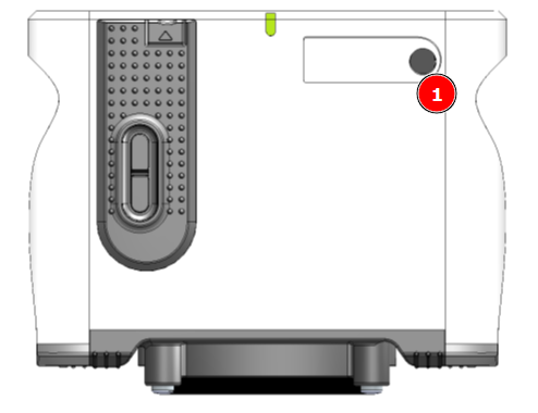
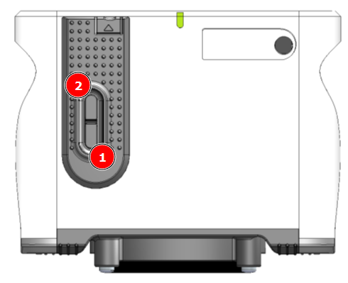
To charge the TAMS, connect the charger output plug to the power input socket (1), then connect the charger to a suitable mains supply.
To reduce charging time and conserve power it is recommended to charge the instrument in powered off state.
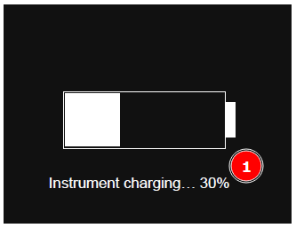
When plugged into power the main screen indicates charging progress (1)
Extra battery sets are available with an external charging station so spare batteries can be charged and swapped in during long or intensive use.
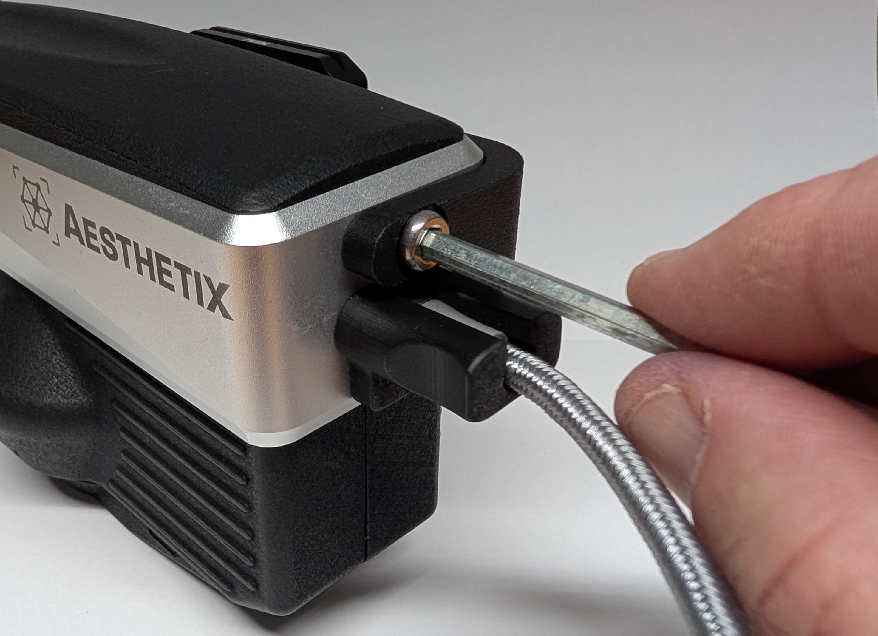
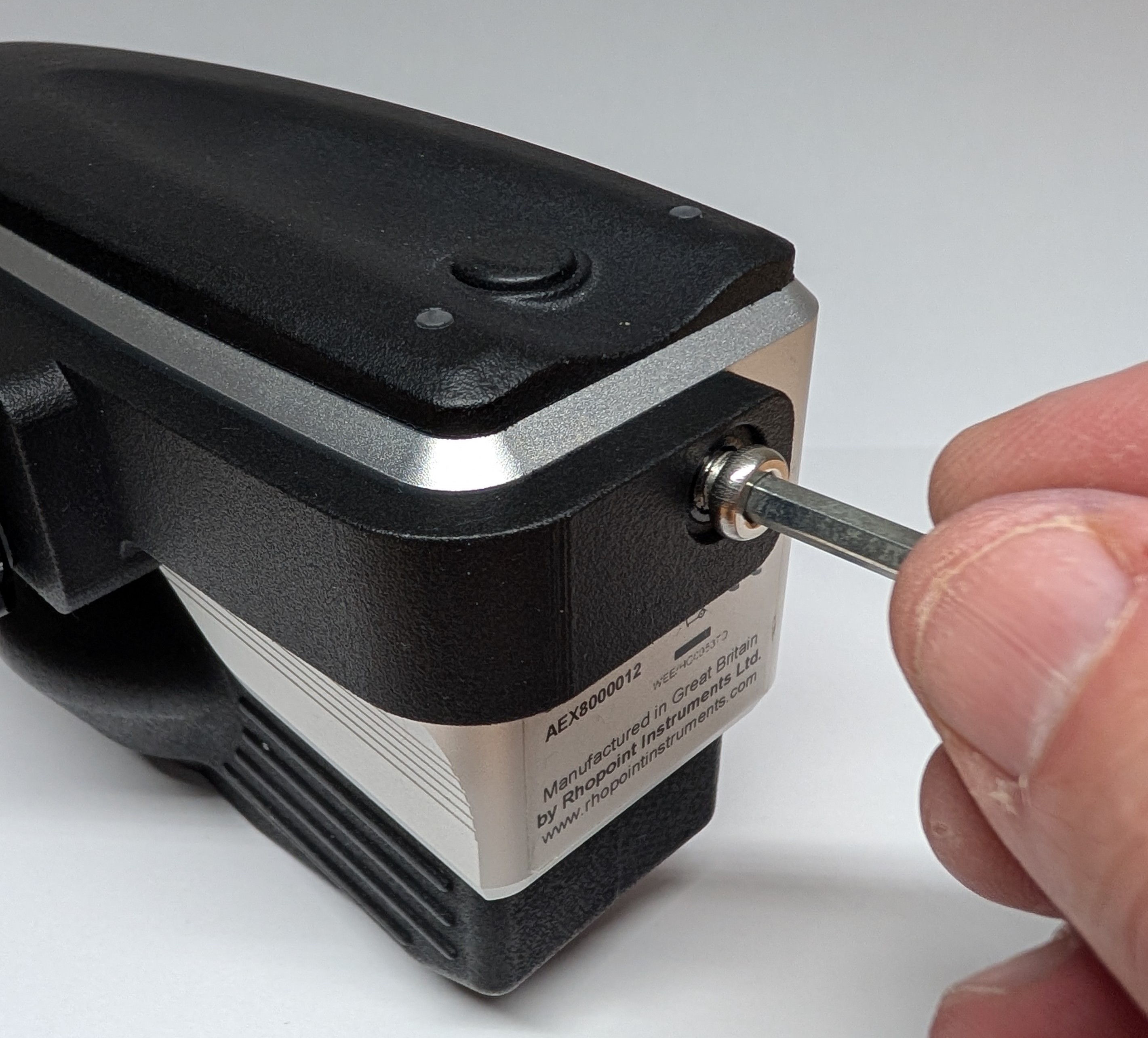
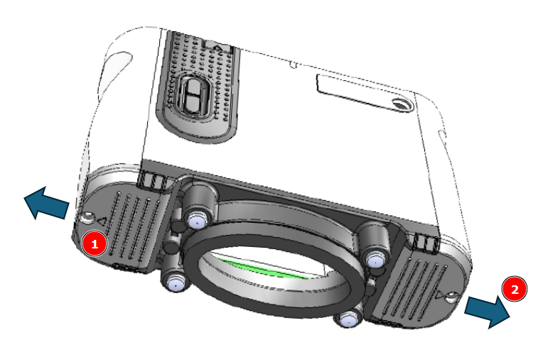
To change batteries, remove the screws (1), slide off each compartment lid (2), withdraw the cells and fit the new ones; the battery bays are keyed so cells can only be inserted in the correct orientation.
To switch the instrument on, press the lower side button (1), after about 25 seconds TAMS is ready; press any key to proceed to the main screen.
 .
.
Soft Reset
If the instrument ever becomes unresponsive, it can be reset by pressing and holding the top side button (2) for about 15 seconds.
Sleep mode
TAMS includes an automatic sleep function to conserve battery power. After a configurable period of inactivity it prepares to switch off, emitting three quick beeps followed by a 10‑second window in which any key press cancels shutdown. If no key is pressed, three normal beeps are emitted and the instrument powers down.
Battery swap behaviour
When new batteries are fitted, TAMS automatically learns their capacity. After a swap it starts up and goes straight to the main screen; a pop‑up confirms the change and instructs to unplug the PSU and wait about 15 seconds while this update completes.
Cleaning the TAMS
Cleaning the TAMS sensor
This page explains how to clean the TAMS optical area and contact surfaces to maintain reliable measurements while avoiding damage to the instrument or sample surfaces.
Safety and general rules
- Do not open the instrument housing or remove any internal covers.
- Always stop measurements and, where possible, switch off the instrument before cleaning.
- Never use household cleaners, abrasive pads or unapproved solvents on any part of TAMS.
Cleaning the sensor lenses and LCD screen
The viewing window and internal optics of TAMS are precision components. They must only be cleaned using a dedicated lens cleaning kit (for example a camera/optical kit with blower, soft lens brush and lens tissues or microfiber cloth).
- Place the instrument on a stable surface with the measurement aperture facing up.
- Inspect the optical window under good lighting for dust, fingerprints or smears.
- Use the blower from the lens kit to remove loose dust and particles; do not use your breath.
- If particles remain, use the soft lens brush from the kit with very light strokes, avoiding any pressure on the window.
- For fingerprints or smears, apply a small amount of lens cleaning fluid to a clean lens tissue/microfiber from the kit.
- Wipe the window gently in straight lines, then dry immediately with a fresh, dry lens tissue.
Do not:
- Spray or drip liquid directly onto the measurement aperture.
- Use paper towels, standard cloths, cotton buds or abrasive wipes.
- Press hard on the window, scrub in circles or reuse dirty tissues.
Cleaning the rubber feet and contact area
The soft rubber feet around the measurement base form the light enclosure and protect the surface being measured. Keep them clean to avoid contamination and sealing issues.
- Wipe the rubber feet and surrounding base gently with a clean, lint‑free cloth slightly dampened with water or mild detergent if needed.
- Remove any paint flakes, dust or debris, taking care not to push contamination into the optical aperture.
- Allow the rubber to dry completely before using TAMS again.
Avoid strong solvents that may swell or damage the rubber material.
Good practice to prevent contamination
- Store TAMS in its case or on the docking station when not in use.
- Avoid placing the measurement base on dusty, abrasive or heavily contaminated surfaces.
- Allow freshly painted surfaces to flash off and harden according to process guidelines before measurement.
- Inspect the optical window regularly; clean promptly if contamination is visible or if measurement stability degrades.
Regular cleaning with a dedicated lens cleaning kit and careful handling will help preserve the optical performance of TAMS and ensure stable, repeatable appearance measurements over the life of the instrument.
Packing List
Packing list
The instrument is supplied as a standard package, complete with all accessories required to calibrate, operate and recharge the unit:
Rhopoint TAMS instrument
Rubber instrument aperture cap
2 × 3.7 V 6800 mAh Li‑Ion batteries
Power supply (9 V / 2 A) for charging
Calibration plate (plastic‑ref, silver‑ref, gloss reference tile)
Quick Start Guide
Lanyard (fitted to instrument)
Protective carry case with custom foam insert
16 GB SD card containing:
- Optimap Reader software
- User manual (PDF)
- Smart Manager data management software
- Release notes (PDF)
- Cleaning cloth
Connecting TAMS to your PC or Network
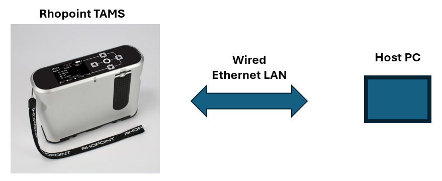
Connecting TAMS via LAN
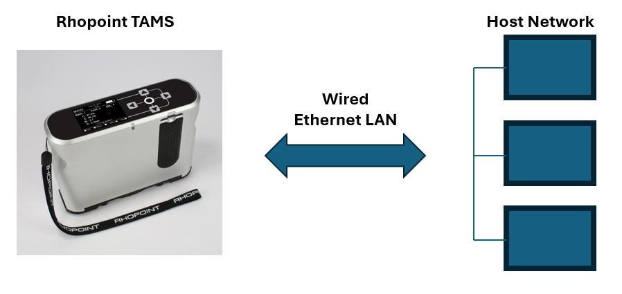
TAMS is connected to a local network using WIFI or via an ethernet cable.
TAMS is supplied with cables and adaptors for connection![image description]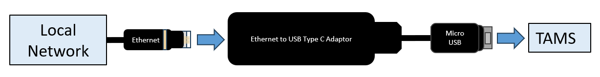
Alternatively the TAMS can be connected to a PC via a wired LAN connection.
Additional cables (supplied) are used to connect to a PC
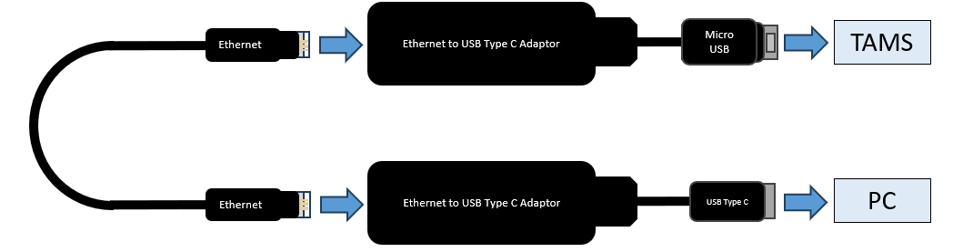
Slide down the door on the TAMS to access the Micro USB port (1)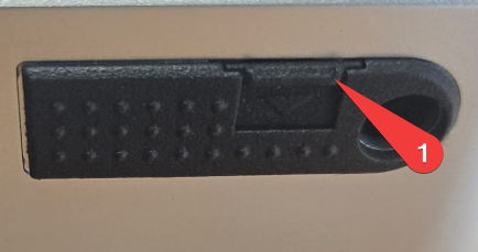
Connecting TAMS via WIFI
To set up wifi TAMS uses an AP mode connection to connect to a local network:
MENU>Admin>Device Settings>Factory>Connectivity>Wifisetup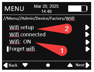
- Switch WIFI to ON
- Click WIFI setup
The TAMS will initialise wifi and wait for a connection.
The green dot (1) indicates the wifi is initialised.
On your PC navigate to Wifi and network settings in windows 11.
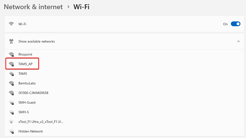
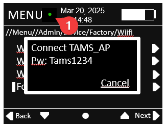
Show available networks then double click on TAMS_AP.
When prompted enter the password Tams1234
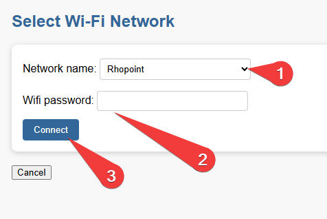
in a browser navigate to the following website- 10.42.0.1
- In the dropdown select the network you wish to connect to
- Enter the wifi password for this network
- Press connect
Once connected the number of green circles (1) indicate the strength of the wifi signal 2- good, 1- OK, 0- poor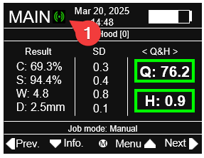
Software
Appearance Elements
Appearance Elements is the main PC application for operating Rhopoint instruments and working with their data. It guides users through connecting a device, running measurements, and viewing results in a clear measurement screen with tables, images and graphs. Dedicated modules focus on different tasks such as gloss, texture and effect pigments, so the interface only shows tools relevant to the active instrument and workflow. Results can be saved to files or a database, and the software can also be started in review‑only mode to explore existing jobs, generate statistics and create reports without a connected instrument.
Appearance Elements (AE)
Elements Hub
Elements Hub is a lightweight connectivity service that makes Rhopoint measurement data available to other software and automation systems. It exposes live values, status and basic control from instruments to external SPC packages, PLCs, robots and cobots using standard connections, so these systems can react to real‑time appearance measurements. By acting as a single hub between Rhopoint devices and third‑party platforms, it simplifies integration projects and avoids custom drivers in every client system.
Elements Hub (EH)
Appearance Elements (AE)
Software
Appearance Elements
Appearance Elements is PC software that runs Rhopoint instruments, guiding the user through measurement, storing results and showing images, maps and graphs. Different modules focus on tasks such as gloss, texture, and effect pigments and the software can also be used just to review and report existing data. Appearance Elements (AE)
Elements Hub
Elements Hub is a connection hub that shares Rhopoint measurement data with other factory systems like SPC software, PLCs and robots. It lets automation cells and quality systems see live results and instrument status without complex custom integration. Elements Hub (EH)
Install AE
Appearance Elements is the Rhopoint software used to operate multiple Rhopoint Instruments.
The latest version of Appearance Elements can be installed from the Rhopoint website.
The functions of Rhopoint Appearance Elements include measurement control, quality control reporting, results analysis, and database storage.
Installation
Visit Rhopoint Instruments Website to download the latest software installer.
Double-click the AppearanceElements.msi package to install the software.
Follow the onscreen instructions.
Start AE Software
Start the software
Double-click the Rhopoint Appearance Elements icon created on the desktop to start the software.
![]()
Rhopoint Appearance Elements desktop icon
Software Update
When connected to the web AE will check Rhopoint Servers for an update.
Additional setup
On the first start, the camera drivers are checked. If the drivers are missing, they will be installed upon confirming the following dialog:
USB camera driver installation
AE Software Update
When connected to the web, Rhopoint Appearance Elements will check for updates.
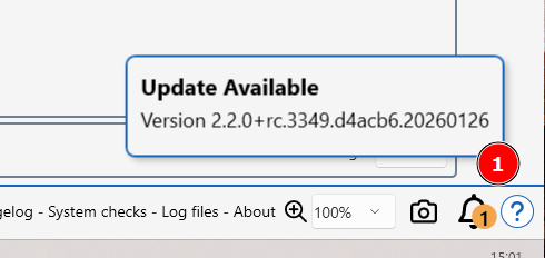
Updated software will include Security updates, bug fixes, an updated manual and feature enhancements.
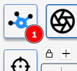
The availability of a new update is indicated as a orange alert (1) on the toolbar.
To install new software click on the alert and follow on-screen instruction.
Installing a new update will not affect saved data or remove licenses.
Update notification
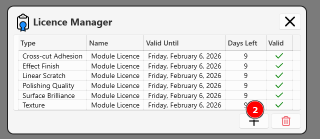
AE License Manager
To install instrument and module licenses, follow these steps:
- Licenses are emailed to you when your instrument is shipped from the Rhopoint factory.
- Download the received licenses onto your PC.
- Click the License Manager (1) button.
- Press the add licenses button (2)
- Select the saved license(s) to install them.
Additional Information
Replacement Licenses:
If you've lost your licenses, you can request them to be resent. Contact sales@rhopointinstruments.com and provide:
- The serial number of your instrument
Demo Licenses:
Rhopoint offers a free 2-week trial for all instruments and modules.
To obtain a demo license, contact sales@rhopointinstruments.com.
Additional Licenses:
To purchase licenses for a new module please contact your regional Rhopoint office, premium authorised distributor or send an email to sales@rhopointinstruments.com.
Connect an Instrument to AE
Click the Device icon (1) to access the connection menu.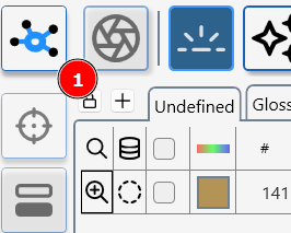

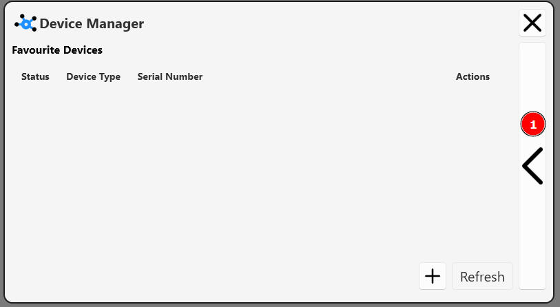
Device Manager- main Screen
Press (1) to add a device via Device Manager add a new device screen
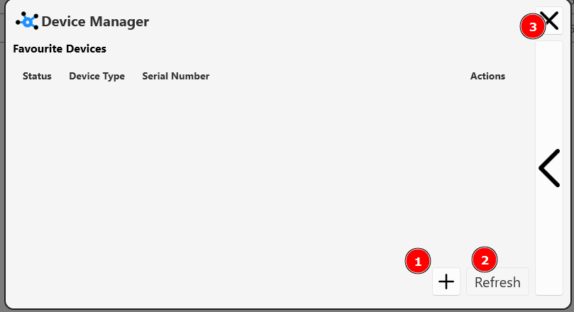
Press (2) to search for previously connected device.
Press (3) to close the device manager window.
If the sensor becomes disconnected, press the refresh button (3) to re-start the sensor discovery process.
Device Manager- add a device screen
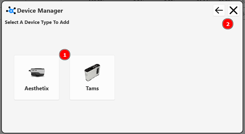
Click on the new device type (1) and follow on screen instructions.
Click (2) exit or return to leave this screen.
Device Manager- main Screen
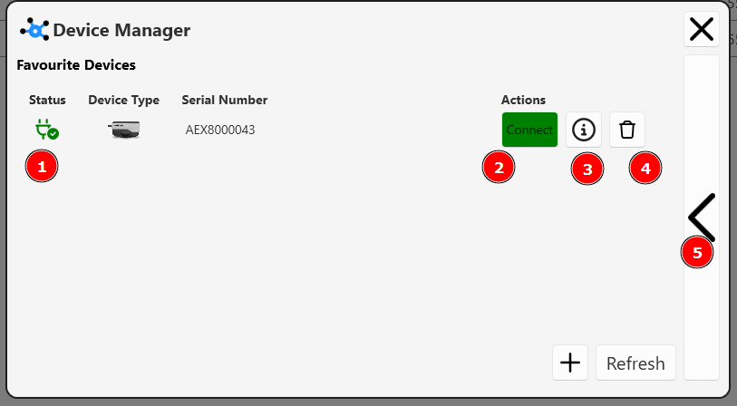
Available devices are listed with a green stats icon (1)
Press (2) to connect to an available device.
Press (3) to access device information.
Press (4) to forget a device.
Press (5) to enter "Viewer mode"
Device Manager- TAMS
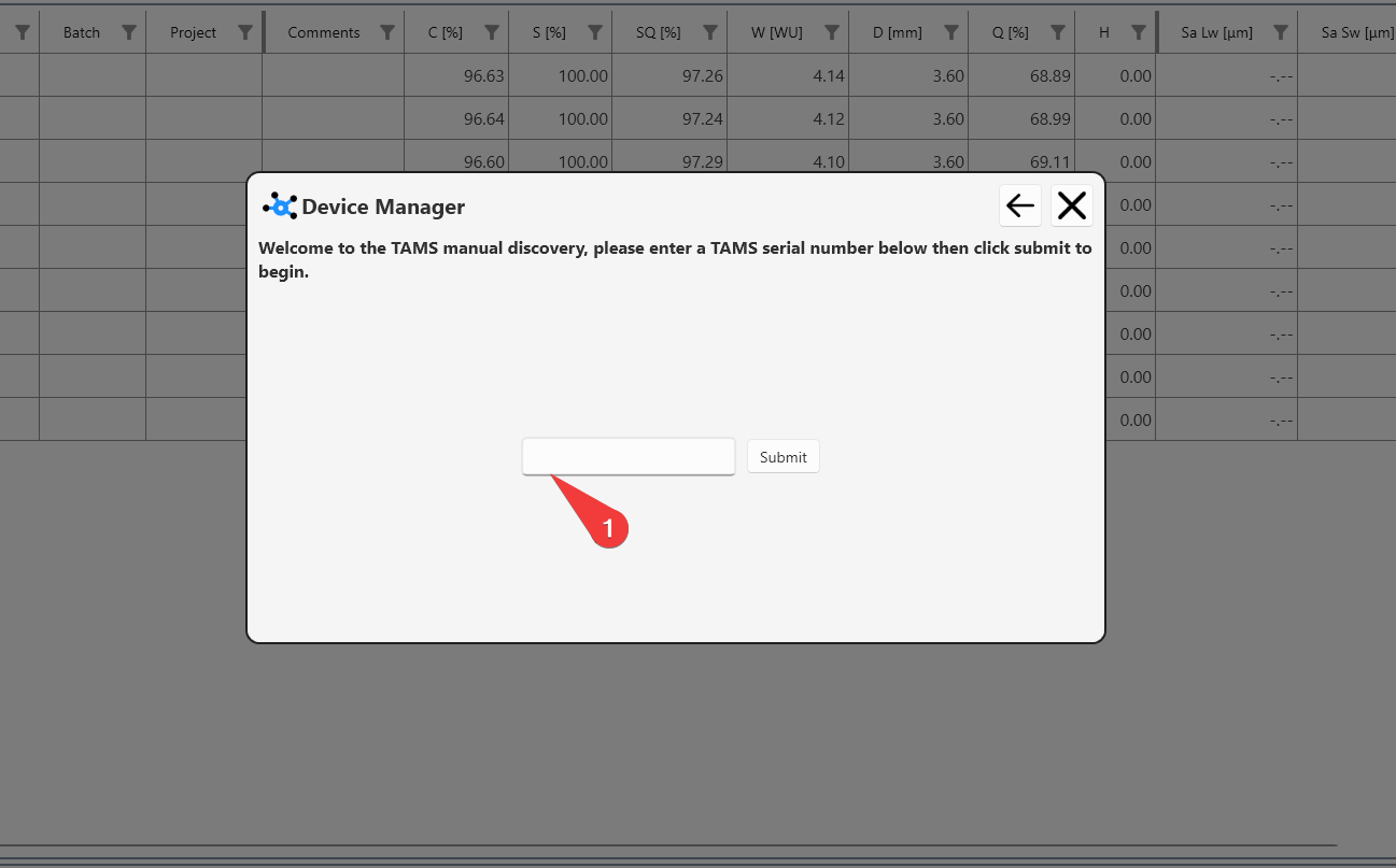
To connect a TAMS, click add a device>TAMs.
Enter the numerical part of the serial number (1) and click submit.
Calibrating an Instrument in AE
To calibrate an instrument in AE click on the calibration icon (1)
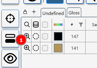
Initiate a measurement(s) in AE
To take a measurement in AE click on the measurment icon (1)
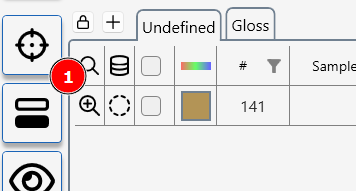
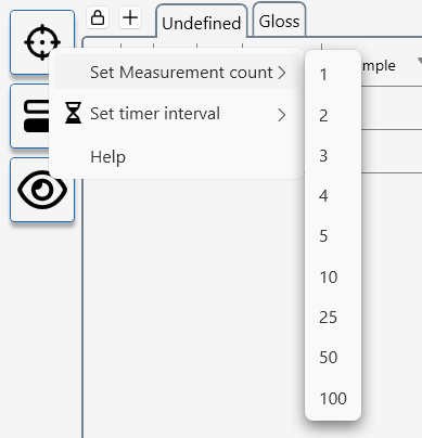
AE can be configured to take multiple measurments at set time intervals.
To access the measurement set up menu- RIGHT click on the neasurment icon
Some instruments and modules have a interactive measurement mode.
This mode uses a live view from a device camera to aid with sample positioning or allows measurement parameters to be fine tuned during the measurement process.
To initiale interactive measuremnt press the interactive measurement icon (1)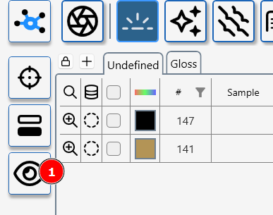
How to use AE without a license
Appearance Elements can be used, license free to interrogate and manipulte previously measured data.
It is not necessary to connect an instrument to access this feature.
Click the Device icon (1) to access the connection menu.
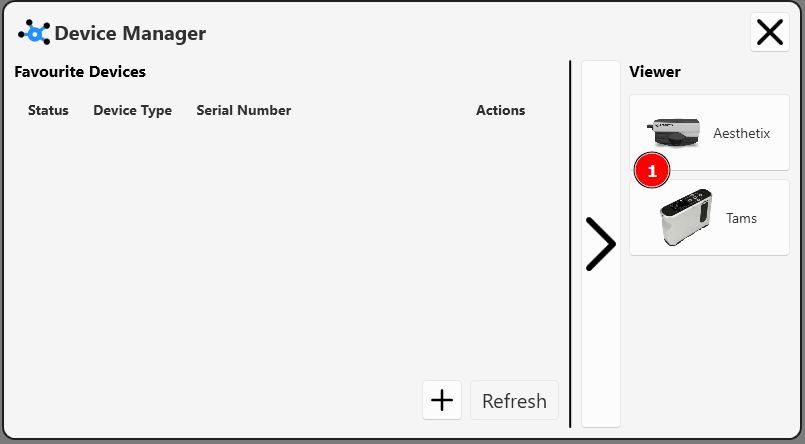
Press the arrow button (1) to enter the viewer menu.
Select the device type required (1)
Navigating the Main Screen
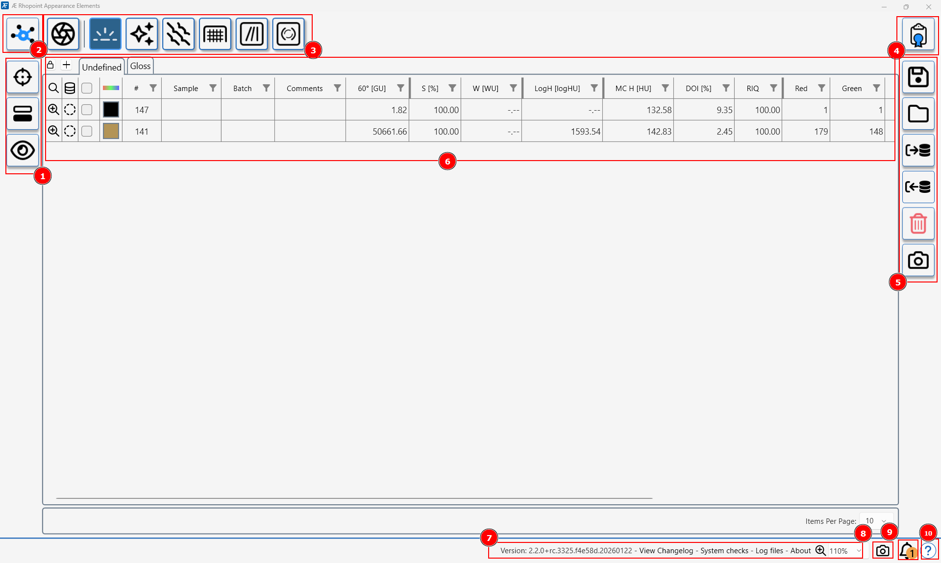
Action Bar
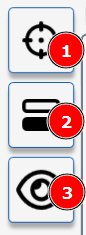
Measure Button
Click here to start a measurement- results will be recorded in the measurement table.
Initiate a measurement(s) in AEA "greyed out" measurement button indicates the license for this module is not present or expired.
Install a new LicenseCalibration
Press to begin Calibration Calibrating an Instrument in AEInteractive Measurement Button
Pressing this button will start an interactive measurement, this includes live views from the Aesthetix camera to allow for sample alignment and adjustment of measurement parameters.
Interactive measurement is not available for certain modules or instruments- this button will not be present in the Action BarTable View
Press this button to toggle the table view. Data Table
Device Manager
This button is used to manage and connect instruments to AE. Connect an Instrument to AE
Module Bar
The module bar in Rhopoint Appearance Elements is where you choose which measurement modules are active in your session. It now supports Aesthetix, Rhopoint TAMS and Rhopoint ID, so what you see depends on both your licenses and the connected instrument.

Module concept
- Each module (for example Surface Brilliance, Effect Finish, Texture, Polishing Quality, TAMS waviness/texture, ID transparency) groups specific metrics and visualisations into a focused workflow. Aesthetix Modules, TAMS Modules
License Manager

Press this icon to access the License Manager
The License Manager installs and manages licenses for instruments and modules in Appearance Elements.
AE License Manager
- Instrument licenses enable live connection and measurement; module licenses enable specific analysis workflows.
- Without a valid license, modules run in viewer‑only mode and measurement buttons are greyed out. How to use AE without a license
You can check the validity of your licenses at licence-check.rhopointservice.com.
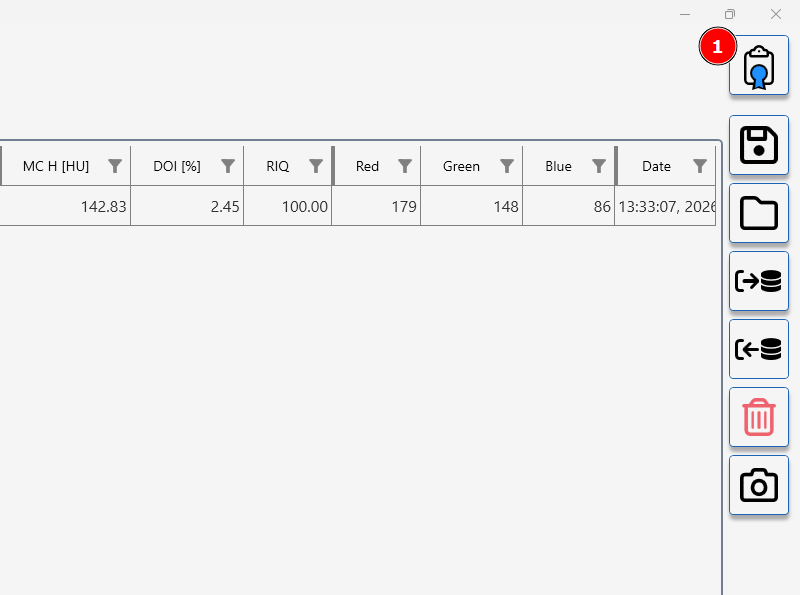
Data Bar

Save and Load Data

Results can be saved (1) or imported (2) from the measurement table.
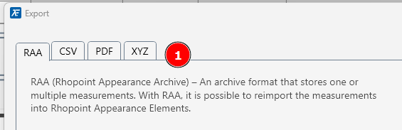
Import/Export options are chosen by clicking on the relevant tab (1)
For analysis in Excel, .csv files can be exported.
Map data can be exported as a .xyz file
Data Table
Data table overview
The data table in Appearance Elements (AE) is the central place where all measurements from connected instruments are listed, organised and edited. Each row represents a single measurement, while columns show key information such as batch name, instrument, module, time stamp and all selected parameters for that result (for example gloss, haze, waviness, roughness or scratch metrics).
Click the magnifier icon for any row in the data table to open that measurement and view all associated content, including images, topographical maps, profiles and graphs.
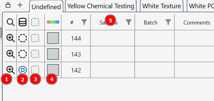
- Use the magnifier lens to see measurement images, graphs and topographical maps.
- Click the database column to add a measurement to the database.
- Select a measurement row(s) for copy and paste, add to the database, or deletion.
- A colour patch represents the measured RGB colour of the surface.
- Right click on column heading to access filter and sort tools.
Viewing Measurement Images and Graphs
Clicking the magnifier icon (1) opens a detailed view of the selected measurement, giving access to all associated images and graphs for that result. This lets you go beyond single numbers and explore how the surface or material actually looks and behaves under the instrument’s optics.
What you can see with the magnifier
Depending on the connected instrument and active module, the magnifier view can include:
- Gloss camera images (Aesthetix / gloss modules): High‑resolution images showing specular reflections, linking gloss, haze and DOI values to visible effects such as halos, streaks or hotspots.
- Topographical maps (Rhopoint TAMS, Aesthetix Texture): 3D height maps and 2D contour views that reveal hills, valleys, orange peel and texture cells, with tools for zoom, rotation and cross‑section profiles.
- Surface images and defect overlays (Aesthetix scratch/defect modules): Observer‑camera images with highlighted scratches, dents or contamination overlaid on the real surface image.
- Profiles and graphs (all instruments): Line profiles, roughness plots, reflectance or appearance curves that show how key metrics change across the measured area.
Why this is useful
- These instrument‑specific images and graphs make it much easier to understand why certain values are high or low, by directly showing the underlying defects, texture, structure or optical behaviour.
- They support rich reporting, allowing you to combine numeric metrics (gloss, haze, waviness, roughness, transparency, scratches, etc.) with visual evidence (images, maps, profiles) when communicating with colleagues, customers or suppliers.
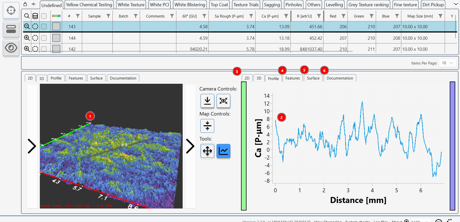
An example image from the Texture module shows a detailed topographial map (1) of the surface and a user selected surface profile (2) from the map.
Clicking on the tabs shows other options 2D surface map (3), watershed feature analysis (4), a colour surface image (5) and a section where the user can take and store photographs of the sample and add further information.
Batching Results
Working with batches in Appearance Elements
Batches in Appearance Elements are used to group related measurements so that data can be analysed, compared and reported more effectively. Batches appear as tabs (1) at the top of the data table, and the batch name is also shown in the Batch column (2) for each measurement row.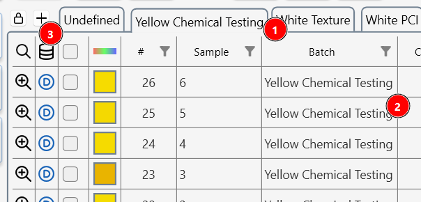
Creating and naming batches
- Click the +(3) button above the data table to open a new batch tab, then enter a name for this batch.
- Alternatively, type a new batch name directly into the Batch column for any measurement; this automatically creates the batch and assigns that measurement to it.
Adding measurements to a batch
- When you take a new measurement while a specific batch tab is active, that measurement is automatically added to the currently selected batch.
- You can also drag and drop existing measurements from the table onto a batch tab to move or copy them into that batch.
Creating a batch from selected measurements
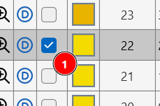
- To build a batch from existing data, select the desired measurements using the selection box (1) in the table.
- Right‑click on the selection and choose Create batch; a new batch is created and all selected measurements are assigned to it.
Statistical Analysis
To perform basic statistical analysis on a number of measurements.
First select the required measurements, then right click in the table.

Click on Combine selected Results
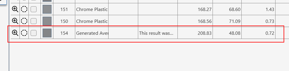
A new line is added to the table- the sample name is set to Generated Average.
This line is the calculated average for all parameters in the table from the selected measurements.
Deleting Data
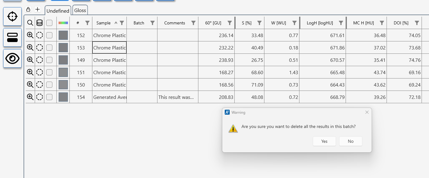
Click the delete icon (1) while no measurements are selected to delete all data from the table.
A dialog window will ask for confirmation.
To delete selected readings
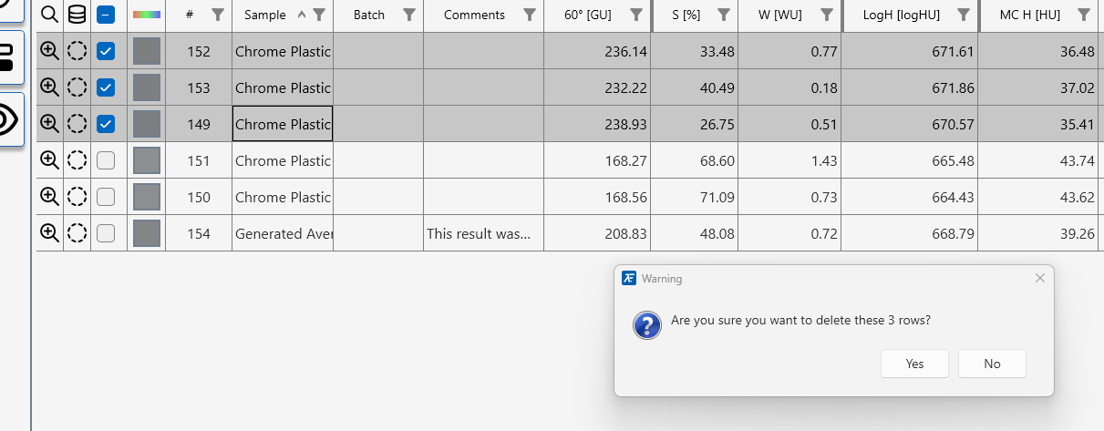
Drag selected rows to the delete icon (1) or press the delete key on you computer keyboard.
Systems Info

- Software version number
- Access changelog.
- Insider program.
- Start system checks.
- Access logfiles
- About information.
- Screen font size.
- Submit a comment.
- Report a bug.
- Take a screen shot
- Notification icon.
- Help menu.
Screen Snip
Notification Alert
Help button
Using the Database
Selected measurements can be saved dynamically in the results database.
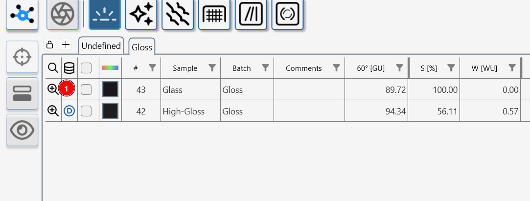
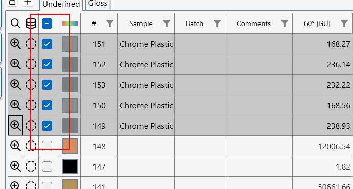
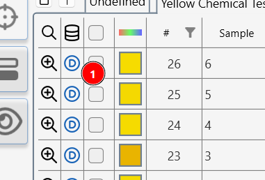
Results saved in the database are marked with a “D” (1)
 ]
]
Measurements marked with a D in the database column are saved in the Appearance Elements database.
To add measurements to the database
- Click on the dashed circle next to the measurement.
- Select multiple measurements in the selection column and click the Save to Database icon.
Several results can be saved in the database by selecting them (1) and clicking the Save to Database icon (2)]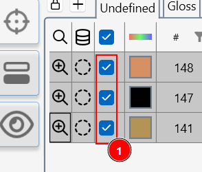
Changes to text or batches made in the Results Table will automatically be updated in the database.
Database viewer
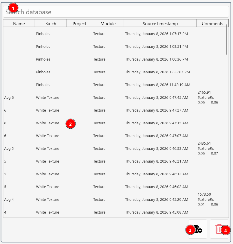
To access the data base view click the Data Base View icon (1)
 .
.
Measurements saved in the database are listed.
- Search the database (1)
- Double click a measurement (2) saved in the database to restore it to the measurement view.
- Highlight an entry and click (3) to add it to the data table.
- Highlight a measurement and click the delete icon (4) to remove it from the database.
Using Aesthetix with AE
Install Appearance Elements
Connect the Aesthetix to AE
The Aesthetix must be connected to an available USB 3.0 port on your PC, Laptop or Windows Tablet.
Configure the Aesthetix Sensor
The Aesthetix can be configured with a standard measurement adaptor, small area/curved surface adaptor, or special jigs or adaptors.
Aesthetix removeable adaptors and jigs
Select a Module
The Rhopoint Aesthetix can be used with multiple software modules to measure different aspects of surface appearance and quality.
Aesthetix Modules
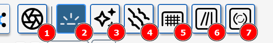
The Module Bar is used to select Measurement Modules.
Visual Demo
A feature which gives the user control over the instrument cameras and light sources.
Read moreSurface Brilliance Module
Measure the gloss, perception gloss, haze, sharpness, DOI and orangepeel on a surface. Read moreEffect Pigment Module
Analyses the appearance of metallic and pearlescent pigments, anodised metals and natural sparkling materials.
Read moreTexture Module
Captures surface roughness, cell amplitude and size, and hill to valley reflectiveness of textured surfaces
Read MoreCross-Cut Adhesion Module
Objectively quantify the results of adhesion strength tests using digital imaging analysis.
Read MoreLinear Scratch Module
Measure the size and area of defects visible in 0/45° lighting conditions. Read MorePolishing Quality Module
Measure the size and area of defects visible in 0/45° lighting conditions.
Read More
Visual demo module
This module is used to manually control Aesthetix light sources and cameras. Surface or gloss images from these screens can be saved with or without overlays.
Surface View Mode
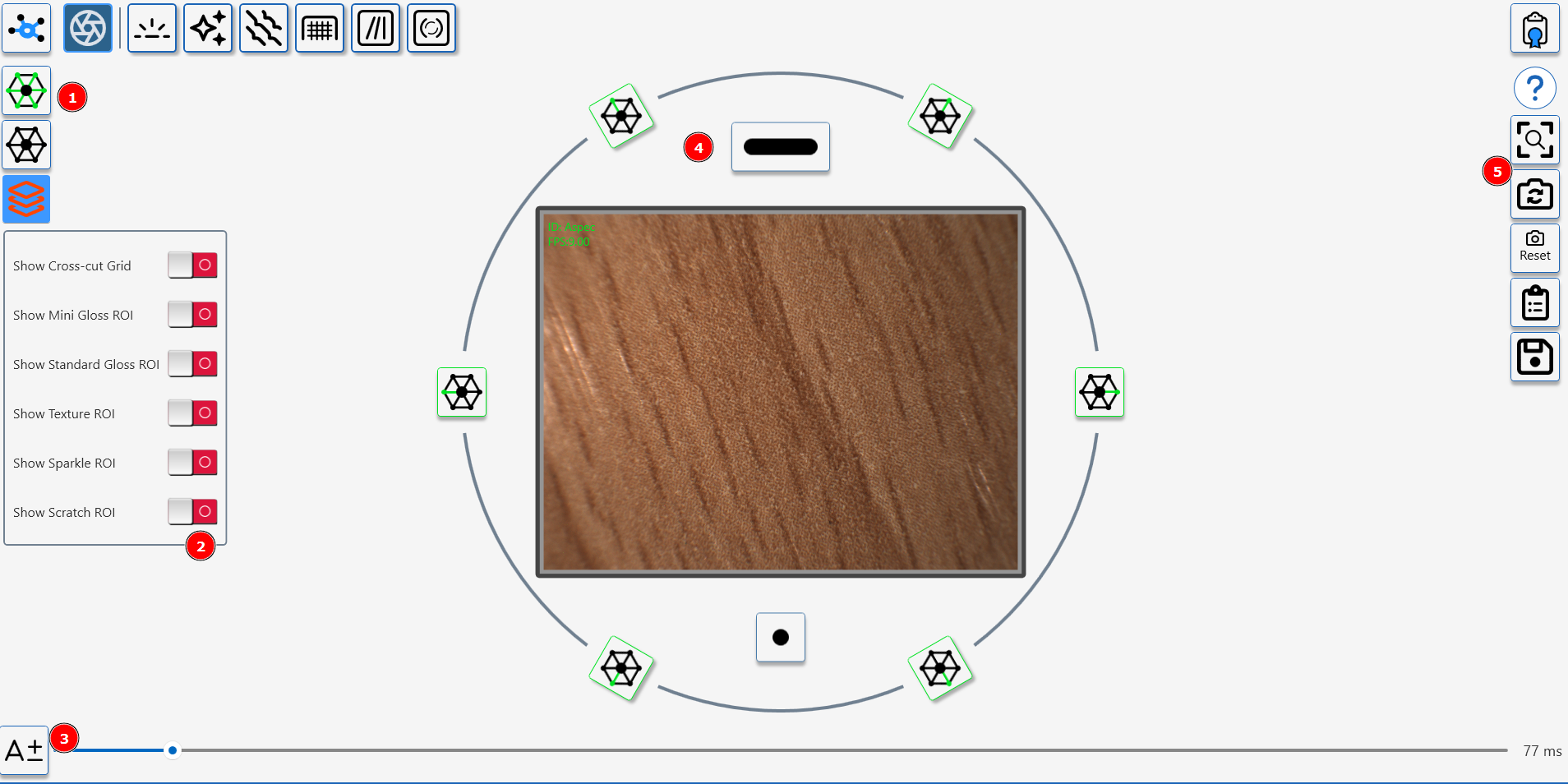
Surface View Controls
- 45 Degree Light- toggle between all on and all off.
- Overlay control- switch on overlays to indicate measurement areas for Aesthetix Modules.
- Camera exposure control, click "A" to activate auto-exposure or use manual slider.
- Individual LED control (Line light, 6 x 45 degree ring lights, 10 degree spotlight )
- Image Controls (Reset view, switch to gloss view, reset camera, copy image to clipboard, save image to file)
Visual demo specular camera
Gloss View Mode
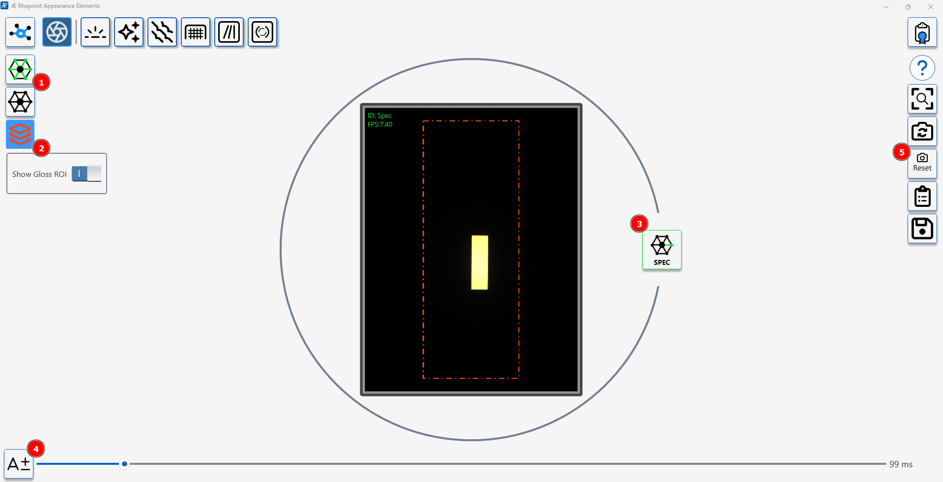
Gloss view controls
- 45 degree light sources toggle on/off.
- Toggle gloss measurment area indicator.
- Toggle gloss light source on/off.
- Camera exposure control, click "A" to activate auto-exposure or use manual slider.
- Image Controls (Reset view, switch to surface view, reset camera, copy image to clipboard, save image to file).
Surface Brilliance
The Surface Brilliance module provides a complete, perception-based evaluation of glossy surfaces by combining gloss, visual gloss, haze, sharpness/DOI, waviness and RGB colour into a single measurement. It is designed to show how “brilliant” or mirror-like a surface appears to the human eye, going far beyond traditional gloss units.
Purpose of this module
Quantify all key contributors to high-gloss appearance, including reflectivity, image sharpness, haze and orange peel/waviness on coated or polished surfaces.
Provide perception-aligned metrics that reduce disputes between suppliers and customers by matching measured values to what people actually see.
Where this module can be used
High-gloss exterior and interior coatings in automotive, commercial vehicles, marine and rail applications.
Premium consumer goods, electronics, furniture, appliances, and other products where mirror-like finishes and brand-defining appearance are critical.
What this module measures
Gloss and Visual Gloss: Conventional gloss values and perception-based gloss scales that better reflect how bright and glossy the surface appears.
Haze, Visual Haze, Sharpness/DOI and Waviness: Metrics for cloudiness, clarity of reflected images and orange peel, plus luminance and RGB colour for full surface characterisation.
How to use this module
In Appearance Elements, select the Surface Brilliance module and choose the appropriate adapter (for example, standard flat panel, curved or small-area adaptor) for your part geometry.
Position the Aesthetix sensor on the surface (or at the defined non-contact distance), run a calibration as recommended, then take one or more measurements and save them to the chosen job, batch or template.
How to interpret the results
Use gloss and Visual Gloss to compare overall brightness and reflectivity; higher values typically indicate a more brilliant, mirror-like finish.
Assess haze, Visual Haze, Sharpness/DOI and Waviness to understand whether defects such as cloudiness, orange peel or loss of image clarity are within acceptable tolerance bands for your product.
Surface Brilliance parameters
| Parameter | Description |
|---|---|
| 60° Gloss | Conventional 60° gloss value indicating how much light is reflected in the specular direction. |
| Visual Gloss | Perception-based gloss scale that predicts how bright and glossy the surface appears to the human eye. |
| Haze and Compensated Haze | Measures light scatter around the main reflection that causes a milky halo and reduces the depth of finish for high gloss coatings. |
| Michelson Contrast Haze MCH | A visual haze metric that quantifies the loss of contrast between the specular highlight and adjacent regions using Michelson contrast, directly reflecting how hazy and sharp the surface appears to the eye |
| Visual Haze | Perception-based haze metrics that describe how hazy the surface looks under different viewing conditions. |
| DOI Distinctness of Image | Quantifies the distinctness of image in the reflection. |
| Sharpness | Quantifies the sharpness and edge definition in the reflection; high values mean crisp, mirror-like images. |
| Waviness | Describes orange peel and surface undulations that distort reflected images over larger spatial scales. |
| RGB colour | Captures colour information (red, green, blue channels) from the surface image for basic colour and appearance tracking. |
How to measure Surface Brilliance
The measurement button is used to start single or multiple measurement that are sent directly to the table.
- Calibrate the sensor
- To access the multiple readings feature, right click on the measurement button.
- Press the measurement button to start.

How to measure Surface Brilliances on surfaces using the interactive measurement feature
The interactive measurement function is a "live" view of the sample surface. It is used to identify particular areas of interest when measuring surface brilliance.
Measurement Procedure
Ensure the sensor is calibrated.
Press the button (1) to activate the interactive measurement feature.

Use the auto-exposure button ( A+/) to optimise the camera exposure for the surface's reflectivity.
Manually adjust exposure if needed using the slider.
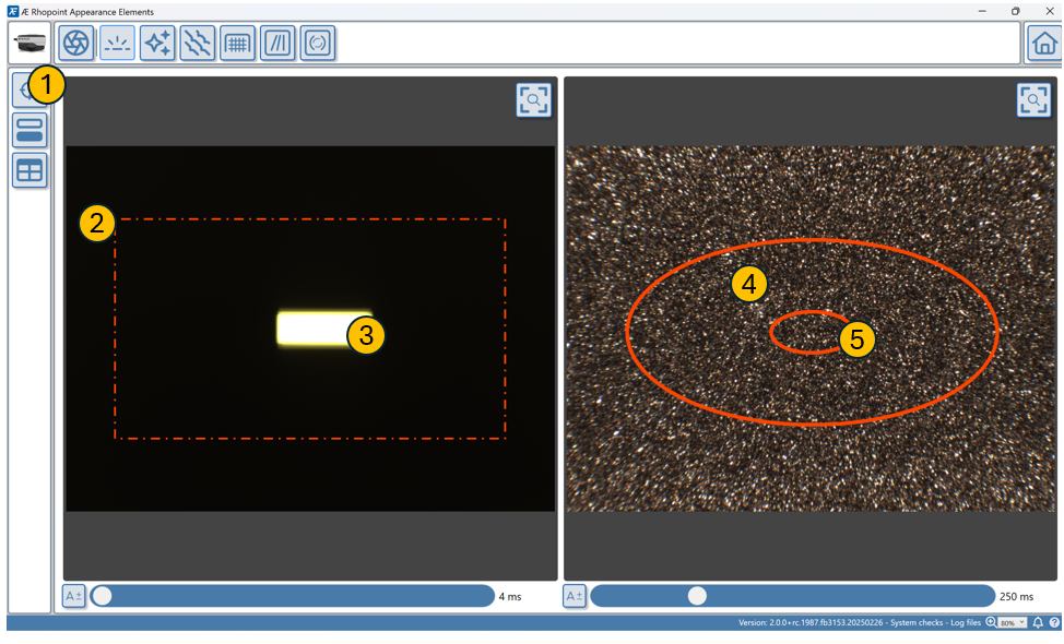
The red dashed area on the live display indicates the target measurement zone for the gloss sensor gloss.
If measuring a curved or uneven surface ensure the gloss reflection (3) is centered in the red dashed box (2) by manually adjusting the orientation of the sample or sensor.
To measure the gloss of a specific area on the surface move the sensor until the required area is covered by the correct red ellipse (4 & 5).
The reflected gloss image on this high gloss coating is intense and sharp & positioned centrally for an accurate gloss measurement.
The surface image shows the area on the surface where the gloss is measured (4- measurement area for standard gloss adaptor & 5- Small area/ curved surface adaptor)
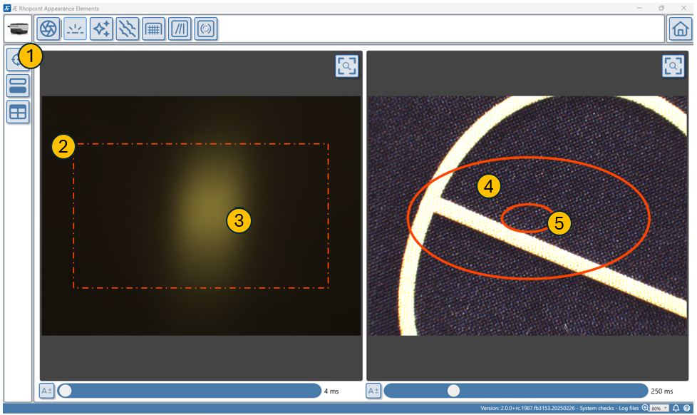
The gloss peak for matt and semi-gloss surfaces is less distinct, for alignment purposes ensure the brightest part of the image is within the red square (2).
Matt surfaces will reflect a image without a peak, ensure the red dashed box on the camera sensor sensor is evenly lit before taking a measurement.
Gloss Measurement Advice
Tips include, when to use Gloss or Visual Gloss, sensor placement and calibration advice.
Measurement Advice
Make sure the instrument is placed flat on the surface.
Regularly calibrate the instrument, once per day is recommended. Calibrating an Instrument in AE
For curved surfaces use the curved surface measurement adapter and interactive measurement feature. Curved Surfaces & Non-Contact Measurement
Measurement Advice—Curved Surfaces
It is not advisable to measure curved surfaces with a radius of <0.5m with the standard gloss adaptor setup.
The instrument is supplied with a curved surface/small parts adaptor which reduces the measurement spot to 2x4 mm- this makes it suitable for curved surfaces.
Gloss- How to Measure Curved Surfaces
Measurement Advice—Complex Parts
For complex shapes or small radius parts it is difficult to correctly position the instrument during measurement - for best results
- Measure non-contact using measurement stand or cobot.
- Use the live positioning feedback to ensure correct positioning.
- For highly reproducible results create 3D printed jigs to position the part in the correct position.
Measurement Advice—Small Areas
It is possible to measure small areas using curved surface/small parts adaptor use the interactive measurement feature to correctly position the instrument before measuring.
Standard Gloss compared to Visual Gloss
- Standard Gloss is does not match customer perception when comparing different coloured materials.
- Gloss measurement alone does not detect surface effects that reduce the appearance quality of high gloss materials- such as Haze, Orange Peel and poor sharpness.
Measurement tip-When to measure with Standard Gloss
Standard gloss measurement is Important for quality control of materials with existing specifications, Aesthetix standard gloss measurements are fully compliant with ISO and ASTM international norms.
Backward compatibility with customers instruments- Aesthetix 60 degree gloss values are perfectly correlated to those supplied by Rhopoint IQ or NG glossmeters or BYK Micro Gloss instruments.
When a quantitative measurement of light reflection is required.
For Gloss measurements that better correlate with perception use VISUAL GLOSS.
For high gloss surfaces- Haze, Sharpness and Waviness are often superior predictors of surface quality than Gloss measurement.
Measurement tip-When Standard Gloss is important
Backwards compatibility with existing measurements : Standard gloss measurements are fully compliant with ISO and ASTM international norms.
Regulatory and Technical Specifications: Many industries have defined standards for gloss levels that need to be met. In such cases, using a glossmeter ensures compliance with these technical specifications.
Interpreting Gloss
Gloss Values and Their Meaning
Gloss is measured in Gloss Units (GU). Here are some typical gloss values for different materials:
| Material | 60-Degree Gloss Value |
|---|---|
| Automotive Clearcoat | 85-95 GU |
| Semi-Gloss Paint | 50-75 GU |
| Satin Paint | 25-35 GU |
| Matte Paint | 5-15 GU |
| Polished Metals | 300-950 GU |
| Perfect Mirror | 1000 GU |
Higher values indicate a more reflective, glossier surface.
Visualising Gloss in Appearance Elements
How to Change Surface Gloss
To change the gloss of a surface:
- Surface Texture: Smoother surfaces generally have higher gloss. Polishing or sanding can increase gloss, while roughening the surface can decrease it.
- Coating Formulation: For coated surfaces, adjust the refractive index of the coating. Higher refractive index materials tend to be glossier.
- Pigmentation: For paints, the type and amount of pigments can affect gloss. Generally, fewer pigments result in higher gloss.
- Application Method: The way a coating is applied can impact gloss. Spray application often yields higher gloss than brush application.
- Curing Conditions: For certain coatings, the curing process can affect final gloss. Proper curing conditions are essential for achieving desired gloss levels.
- Substrate: The underlying material can influence gloss. A smoother substrate often results in a glossier finish.
Remember that changing gloss may affect other surface properties, so consider the overall impact on the product's performance and appearance.
How to Measure Curved Surfaces
Measuring the relfected atributes of curved surfaces is challenging (or impossible) with a standard glossmeter. The Rhopoint Aesthetix addresses these issues with its advanced optical design, optional small measurement beam and interactive measurement feature.
Preparation
Adaptor Selection:
- Replace the standard flat surface adaptor with the curved surface/small parts adaptor, Novo-Curve Adaptor or custom 3D printed Jig. This adaptor reduces the beam size, making it suitable for curved surfaces.
Aesthetix removeable adaptors and jigs
- To attach the adaptor:
- Remove the standard adaptor by pulling it off (magnetically attached).
- Attach the curved surface adaptor securely in its place.
Calibration:
- Recalibrate the instrument after changing adaptors to ensure accurate measurements. Use the supplied calibration tile certified to meet traceability standards.
Positioning Tools (Optional):
- For repeatable measurements on small or complex parts, use bespoke 3D-printed jigs or a laboratory stand. These tools help maintain consistent positioning during measurement.
Measurement Procedure
Using the Curved Surface Adaptor
Instrument Placement:
- Use the interactive measurement feature to ensure that the measurement beam is centered on the reflection image. Misalignment can lead to inaccurate results.
How to measure Surface Brilliance
- Use the interactive measurement feature to ensure that the measurement beam is centered on the reflection image. Misalignment can lead to inaccurate results.
Measurement Execution:
- Press the measurement button once alignment is confirmed. The Aesthetix will capture data for gloss, haze, DOI, and other parameters simultaneously.
Non-Contact Measurement (Optional)
For fragile or delicate surfaces:
- Mount the Aesthetix on a height-adjustable stand or integrate it into a COBOT system. Ensure that the focal distance is maintained at 10 mm ± 0.5 mm from the target surface.
- Follow steps for live alignment and execute measurements as described above.
Tips for Accurate Measurement
- Avoid measuring surfaces with a radius smaller than 0.5 m using standard adaptors; always use the curved surface adaptor for such cases.
- For highly complex shapes, consider non-contact measurement methods combined with custom jigs or COBOT systems for precise alignment.
- Regularly calibrate the instrument to maintain accuracy, especially after changing adaptors or environmental conditions.
Applications
The Rhopoint Aesthetix excels in industries requiring precision appearance control of curved components, such as:
- Automotive (e.g., chrome trims, high-gloss paint finishes)
- Medical devices (e.g., orthopedic implants)
- Consumer electronics (e.g., buttons, casings)
- Pharmaceuticals and confectionery (e.g., pills, candy coatings).
By following these steps and leveraging its advanced features, you can achieve reliable and repeatable measurements of curved surfaces with your Rhopoint Aesthetix instrument.
Visual Gloss: for enhanced correlation with human perception
When to use Visual Gloss GU compared to Standard Gloss GU
Visual gloss is better suited for applications where human perception is crucial, standard gloss is useful when compliance to a standard is key or measurements need to match historic specifications.
Balancing between these two methods can be essential depending on the specific requirements of the project or product
Measurement tip-When Visual Gloss is important
Subjective Perception is Key: If the goal is to understand how people perceive the glossiness of a surface under real-world conditions, VG is more appropriate.
This is crucial in industries where the aesthetic and visual appeal are critical, such as in automotive finishes, furniture, consumer electronics, and interior design. Both measurements are visible simultaneously in Rhopoint Appearance Elements software.
Product Development and Marketing: When developing products where the consumer's perception influences their decision to purchase, VG can provide insights into how potential buyers might view the product under typical use conditions.
Quality Control: If the product quality is judged visually by consumers, VG assessments can help ensure consistency in how products are perceived in the marketplace.
Surface Haze Measurement Guide
What is Haze?
Haze refers to the scattering of light by a surface that causes a reduction in the contrast of a reflected image. It results in a milky appearance which can reduce the perceived depth and clarity of a finish[^1]. Haze is often caused by microscopic surface irregularities, contaminants, coating defects, or subsurface imperfections that scatter light in various directions[^1].
How Aesthetix Measures Haze
The Aesthetix measures haze using an advanced imaging technique:
- It captures a high-dynamic-range (HDR) image of the surface reflection
- The system analyzes the light distribution around the main specular reflection
- It quantifies the amount of scattered light in specific angular regions
This method allows for a more comprehensive assessment of haze compared to traditional haze meters.
Haze Metrics Provided by Aesthetix
The Aesthetix provides several haze-related metrics:
- LogH (LogHaze): Logarithmic haze value in logHU
- LogH C: Logarithmic haze with background compensation in logHU
- Haze C: Haze with background compensation in HU
- MC H (Contrast Haze): Calibrated contrast haze value in HU
- Visual Haze Indoors: Visual haze value for indoor viewing conditions in VHU
- Visual Haze Outside: Visual haze value for outdoor viewing conditions in VHU
Comparison and Usage
- LogH and LogH C provide logarithmic scales, which can be useful for materials with a wide range of haze values.
- Haze C and MC H offer linear scales with background compensation, providing more accurate results for colored or textured surfaces.
- Visual Haze metrics (Indoors and Outside) are perception-based measurements that correlate closely with human observation under different lighting conditions.
For most applications, Visual Haze metrics are recommended as they best represent how haze is perceived by human observers. Use Visual Haze Indoors for products primarily viewed indoors, and Visual Haze Outside for products exposed to outdoor lighting[^1].
For technical or research applications where comparison to traditional haze measurements is needed, LogH or Haze C may be more appropriate.
Visualizing Haze in Appearance Elements
Altering Surface Haze
To alter the haze of a surface:
- Surface Polishing: Fine polishing can reduce surface irregularities and decrease haze.
- Coating Formulation: Adjust the coating formula to include additives that promote smoother surface formation or reduce micro-texture.
- Application Technique: Optimize spray patterns, drying conditions, and curing processes to minimize surface irregularities during coating application.
- Surface Cleaning: Thoroughly clean the surface to remove contaminants that may contribute to haze.
- Substrate Preparation: Ensure the underlying substrate is smooth and free of defects that could telegraph through the coating.
- Post-Treatment: For some materials, post-application treatments like heat or UV curing can help reduce haze by promoting better surface leveling.
- Environmental Control: Control humidity and temperature during application and curing to prevent issues like blushing that can increase haze.
Remember that altering haze may affect other surface properties, so consider the overall impact on the product's appearance and performance when making changes.
- Haze : Logarithmic haze value in logHU
- LogH C: Logarithmic haze with background compensation in logHU
- Haze C: Haze with background compensation in HU
- MC H (Contrast Haze): Calibrated contrast haze value in HU
- Visual Haze Indoors: Visual haze value for indoor viewing conditions in VHU
- Visual Haze Outside: Visual haze value for outdoor viewing conditions in VHU
Comparison and Usage
- LogH and LogH C provide logarithmic scales, which can be useful for materials with a wide range of haze values.
- Haze C and MC H offer linear scales with background compensation, providing more accurate results for colored or textured surfaces.
- Visual Haze metrics (Indoors and Outside) are perception-based measurements that correlate closely with human observation under different lighting conditions.
For most applications, Visual Haze metrics are recommended as they best represent how haze is perceived by human observers. Use Visual Haze Indoors for products primarily viewed indoors, and Visual Haze Outside for products exposed to outdoor lighting[^1].
For technical or research applications where comparison to traditional haze measurements is needed, LogH or Haze C may be more appropriate.
Visualizing Haze in Appearance Elements
Altering Surface Haze
To alter the haze of a surface:
- Surface Polishing: Fine polishing can reduce surface irregularities and decrease haze.
- Coating Formulation: Adjust the coating formula to include additives that promote smoother surface formation or reduce micro-texture.
- Application Technique: Optimize spray patterns, drying conditions, and curing processes to minimize surface irregularities during coating application.
- Surface Cleaning: Thoroughly clean the surface to remove contaminants that may contribute to haze.
- Substrate Preparation: Ensure the underlying substrate is smooth and free of defects that could telegraph through the coating.
- Post-Treatment: For some materials, post-application treatments like heat or UV curing can help reduce haze by promoting better surface leveling.
- Environmental Control: Control humidity and temperature during application and curing to prevent issues like blushing that can increase haze.
Remember that altering haze may affect other surface properties, so consider the overall impact on the product's appearance and performance when making changes.
Visual Haze: predict haze visibilty in different viewing environments
NEW Visual Haze measurement is more sensitive and more consistent with human perception because it accounts for illumination conditions and background paint colour.
Visual haze is calculated considering the luminosity of the background colour and the luminosity of the near specular reflection (Haze).
Two values are provided to account Haze visibility in two different viewing conditions, indoor viewing compared to outdoor viewing in strong sunlight.
.png)
Two panels with identical reflective properties but Haziness is not visible on the white material. Visual Haze records the perceived haziness.
Visual Haze matches human perception and used to avoid unnecessary material rejections and over processing.
Visual Haze VH Indoor Vhin and Visual Haze Outdoor Vhout
Haze effects are amplified in strong sunlight- swirls whirls and holograms which are not visible in indoor conditions are prominent when illuminated by a high intensity light-source.
.png)
Surface Defects which are not detected by technical haze (LogH C) are very visible in strong sunlight.
The Aesthetix can predict the visibility of haze, scratches and polishing marks in workshop and sunny outdoor conditions.
| Conditions | Surface illumination | Specular Illumination | |
|---|---|---|---|
| VHin | Standard indoor lighting | 0.5k Lux | 25k cd/m2 |
| VHout | Sunny day- clear sky | 100k Lux | 1.6m cd/m2 |
| Haze | Surface | Description/Perception |
|---|---|---|
| <50 Hu (Indoor or outdoor) | High Quality Surface | Almost perfect surface- haze not visible under normal viewing conditions. |
| 50-100 | Ultra Low Haze Surface | Good depth of finish- Barely visible halo around reflected light sources. |
| 100-250 | Visible Haze | Depth of finish is compromised- swirls and polishing marks are visible |
| 250-300 | Hazy Surface | Poor quality finish |
| 300-500 | Poor Quality Surface | Prominent halos, holograms or polish marks. Poor depth of finish |
Interpreting MC Michelson Contrast Haze
Haze refers to the scattering of light by a surface that causes a reduction in the contrast of a reflected image. It results in a milky appearance which can reducing the perceived depth of the finish
Michelson Contrast Haze- MC H (HU)
The MC H parameter, or Michelson Contrast Haze, in the Rhopoint Aesthetix is a haze metric based on Michelson contrast.
It quantifies the difference between the luminance of the specular highlight and the adjacent off-specular regions. This method provides insights into how surface microstructure affects visual haze, which traditional haze measurements may overlook.The MC H parameter, or Michelson Contrast Haze, in the Rhopoint Aesthetix is a haze metric based on Michelson contrast. It quantifies the difference between the luminance of the specular highlight and the adjacent off-specular regions.
This method provides insights into how surface microstructure affects visual haze, which traditional haze measurements may overlook.
Waviness Measurement Guide
What is Waviness?
Waviness refers to gentle undulations or waves visible on a surface that is meant to be smooth. In coated surfaces, this effect is often called "orange peel" because the texture resembles the skin of an orange.
Waviness is an optical effect caused by large structures (0.1-10mm) on the surface of the material.
For high gloss finishes, excessive waviness reduces the perceived quality by disrupting the uniformity and clarity of reflected images.
Waviness is a key parameter when observers judge the appearance quality of high gloss coatings. A smoother, low waviness coating is perceived as higher quality compared to a similar surface with more surface texture (higher waviness).
How Aesthetix Measures Waviness
The Aesthetix measures waviness by quantifying the distortion in a 25mm straight line reflected in the material surface.
Waviness Values and Their Meaning
The Aesthetix waviness scale is highly correlated to Rhopoint TAMS waviness - a measurement parameter derived from multiple human perception trials.
The value quantifies the visual impact of orange peel observed in high gloss coatings at a viewing distance of 1.5m.
This value has been proven effective for quantifying orange peel in sectors such as automotive, yacht Coatings, powder coatings and high quality furniture.
Waviness values and their meanings:
- 2 WU: Piano Finish - Very smooth with no visible waviness. Imparts a feeling of very high quality.
- 2-5 WU: Low orange peel - Smooth finish, orange peel is barely visible with a good or neutral impact on judgement of surface finish.
- 5-10 WU: Standard Orange Peel - Surface with moderate orange-peel which is visible and is a factor when judging finish quality, especially on high contrast colors (black).
- 10-15 WU: High Orange peel - Surface with prominent orange peel which has a negative impact on surface quality judgement.
Changing the Waviness of a Surface
To change the waviness of a surface:
- Improve Application Technique: Proper spraying distance, angle, and technique can reduce uneven paint distribution that leads to orange peel.
- Adjust Paint Viscosity: Use paint with the correct viscosity for better flow and leveling, reducing bumpy finishes.
- Control Environmental Factors: Maintain appropriate humidity and temperature during application and drying to prevent uneven drying that can cause orange peel.
- Enhance Surface Preparation: Adequate sanding and cleaning of the surface before painting can minimize imperfections that contribute to waviness.
- Allow Proper Curing Time: Sufficient drying time between coats can result in a more even surface texture.
- Optimize Equipment Settings: Use the correct nozzle size and pressure settings on spray guns for proper paint atomization.
- Address Substrate Issues: Improve the underlying material quality, as texture in the substrate can telegraph through the coating layers, causing visible orange peel[^1].
Remember that changing waviness may affect other surface properties, so consider the overall impact on the product's appearance and performance when making adjustments.
DOI & Sharpness Measurement Guide
| DOI Units | Description |
|---|---|
| 0-50 % | No discernible reflected image. |
| 50-70 % | Low DOI, a reflected image is barely visible. |
| 70-90 % | Moderate DOI, a distinct reflected image is visible. |
| 90-95 % | High DOI, showing a very clear and distinct reflected image. |
| 95-100 % | Very high DOI, indicating an exceptionally clear reflection. |
What are sharpness and DOI?
How does Aesthetix these values?
How do these values compare, which one should i use for my application?
How Can I visualise DOI/Sharpness Using Appearance Elements?
How can I change the DOI and Sharpness of a surface?
Sharpness and DOI
Sharpness and Distinctness of Image (DOI) are related measurements that quantify the clarity and definition of reflections on a surface.
Sharpness
Sharpness specifically assesses the clarity and definition of edges within a reflected image. It is measured on a scale from 0 to 100 Sharpness Units (SU), where higher values indicate clearer, sharper reflections[^1].
Distinctness of Image (DOI)
DOI evaluates the overall clarity and distinctness of the entire reflected image. It quantifies how clearly and undistorted an image is reflected off a surface[^1].
Aesthetix Measurement Method
The Aesthetix measures sharpness by:
- Capturing a high-resolution image of a light source reflected on the sample surface using its camera sensor
- Analyzing the sharpness of edges in this reflected image
- Deriving a sharpness value that correlates with human visual perception[^1]
For DOI, the Aesthetix likely uses a similar image-based approach, analyzing the overall clarity of the reflected image rather than focusing specifically on edge sharpness.
Comparison and Usage
Sharpness is generally considered more advanced and sensitive than traditional DOI measurements, especially for high-quality surfaces[^1].
- Sharpness provides more detailed information about edge clarity in reflections
- Sharpness correlates better with human visual perception
- Sharpness can detect subtle differences in very high-quality surfaces that DOI may miss
For most modern applications, especially those involving high-gloss or high-quality surfaces, sharpness is recommended over DOI. However, DOI may still be used for backwards compatibility with existing specifications or standards[^1].
Visualizing in Appearance Elements
To visualize sharpness/DOI in Appearance Elements:
- Use the live view feature from the gloss camera
- Switch to the gloss camera view using the switch camera icon
- Use auto-exposure to optimize for the surface's reflectivity
- Manually adjust exposure if needed
- Control the specular light source, line light, and spotlight as needed[^2]
The software will display sharpness/DOI values and may provide visual representations of the reflected image quality.
Changing DOI and Sharpness
To improve DOI and sharpness of a surface:
- Enhance surface smoothness through finer polishing or sanding techniques
- Optimize coating formulations to promote better leveling and flow
- Improve application methods to minimize orange peel and other texture issues
- Ensure proper curing conditions to allow coatings to level optimally
- Use high-quality basecoats or primers to create a smoother foundation
- For plastic parts, optimize molding conditions to reduce surface defects
- Consider using flow additives in coatings to promote better leveling
Remember that changes to improve sharpness/DOI may affect other surface properties, so consider the overall impact on the product's appearance and performance[^1].
Start writing your section content here.
Effect Finish Module
The Effect Finish module characterises coatings containing metallic, effect pigments by measuring sparkle, graininess, waviness, gloss and RGB colour, so you can control how dynamic, coarse and colourful the finish appears under real viewing conditions. It links image-based sparkle metrics with conventional gloss measurements to describe effect finishes in a way that closely follows human visual perception.
Purpose of this module
- Quantify the key visual attributes of effect coatings, including sparkle density and visibility, graininess, waviness/orange peel, gloss and colour, under defined geometries.
- Provide perception-aligned parameters for effect finishes, helping formulators and OEMs specify and agree on target appearance for metallic and pearlescent systems.
Where this module can be used
- Automotive and commercial vehicle exterior and interior parts using metallic or pearlescent basecoats, tricoats or coloured effect layers.
- Consumer electronics, appliances, packaging, cosmetics and other products that rely on controlled sparkle, graininess and overall surface character to support branding and premium appearance.
What this module measures
- Sparkle metrics (Density, Area, Brightness, Visibility in RGB channels at 10° and 45°) that describe how many sparkle points are visible, how large they are and how bright they appear from different angles.
- Graininess, waviness, gloss and RGB colour, giving a combined description of coarseness, orange peel and overall reflectivity/colour of the effect finish.
How to use this module
- In Appearance Elements, select the Effect Finish module, choose the appropriate fixture or stand for your sample geometry, and perform the recommended calibration on the supplied reference standard.
- Place the Aesthetix sensor over the area of interest, trigger one or more measurements, and store the results in the relevant job, batch or template for later comparison.
How to interpret the results
- Use sparkle Density, Area, Brightness and Visibility (at 10° and 45°) to judge how intense, coarse and angle-dependent the sparkle effect appears compared to target or reference panels.
- Combine graininess, waviness, gloss and RGB data to determine whether the overall coarseness, orange peel and colour of the effect coating fall within agreed appearance specifications for your application.
Effect Finish Parameters
| Index | Description (Effect Finish module) |
|---|---|
| 60° | 60° Gloss; overall specular reflectance level of the effect coating. |
| Waviness | Waviness of the effect finish, describing large‑scale distortion of reflections. |
| Graininess | Perceived coarseness or fineness of the metallic/effect flake structure in the coating. |
| Density (10°) | Number of visible sparkle points per 100 mm² area near 10°, indicating how densely flakes sparkle head‑on. |
| Area (10°) | Average sparkle size near 10°, describing the typical area of individual sparkle elements. |
| Brightness (10°) | Average luminance of sparkle points near 10°, describing how bright the sparkles appear head‑on. |
| Visibility (10°) | Average perceived brightness of sparkle elements near 10°, considering their visibility and the background colour of the material. |
| Density (45°) | Number of visible sparkle points per 100 mm² area at 45°, indicating flake activity at the side view. |
| Area (45°) | Average sparkle size at 45°, describing the typical area of individual sparkle elements off‑specular. |
| Brightness (45°) | Average luminance of sparkle points at 45°, describing perceived sparkle brightness from the side. |
| Visibility (45°) | Average perceived brightness of sparkle elements at 45°, considering their visibility and the background colour of the material. |
| SpR (10°) | Red‑channel sparkle intensity measured close to the viewing direction at 10°. |
| SpG (10°) | Green‑channel sparkle intensity measured close to the viewing direction at 10°. |
| SpB (10°) | Blue‑channel sparkle intensity measured close to the viewing direction at 10°. |
| SpR (45°) | Red‑channel sparkle intensity measured at the off‑specular 45° viewing direction. |
| SpG (45°) | Green‑channel sparkle intensity measured at the off‑specular 45° viewing direction. |
| SpB (45°) | Blue‑channel sparkle intensity measured at the off‑specular 45° viewing direction. |
| R | Average red‑channel surface colour of the effect finish (RGB). |
| G | Average green‑channel surface colour of the effect finish (RGB). |
| B | Average blue‑channel surface colour of the effect finish (RGB). |
Interpreting Effect Finish Parameters
How Does Aesthetix Measure Sparkle and Graininess?
The Aesthetix measures sparkle and graininess using advanced imaging techniques that capture surface reflectance under specific lighting conditions.
- Sparkle Measurement: Sparkle is quantified by identifying and analyzing bright points of light (sparkle points) that are significantly brighter than their surroundings under directional illumination. The system captures high-dynamic-range images using multiple light sources at 45° and a single image at 10° angles. The visibility, density, and size of these sparkle points are calculated based on contrast thresholds, luminance, and spatial distribution.
- Graininess Measurement: Graininess is assessed under diffuse lighting conditions. The software analyzes the spatial variation in the luminance factor of the surface, focusing on intermediate spatial frequencies. This captures the non-uniform, granular texture perceived as graininess.
Measurements Provided by Aesthetix for Sparkle and Graininess
Sparkle Metrics:
- Sparkle Density: Number of visible sparkle points per 100 mm².
- Sparkle Visibility: Average intensity of visible sparkle points relative to the background.
- Sparkle Area: Average size of individual sparkle points in square micrometers.
Graininess Metrics:
- Graininess Value (G): Quantifies the perceived coarseness of a surface under diffuse lighting, adjusted for luminance levels.
Comparison and Application:
- Use Sparkle Density and Visibility for applications where the brightness and concentration of sparkle points are critical (e.g., automotive coatings or cosmetics).
- Use Graininess Value for assessing surface uniformity in diffuse lighting, especially in applications like interior finishes or textured coatings.
For most applications, both metrics provide complementary insights into surface appearance. Choose based on whether directional (sparkle) or diffuse (graininess) lighting conditions dominate in the product's end-use environment.
Visualizing Sparkle and Graininess Using Appearance Elements
The Rhopoint Appearance Elements software allows detailed visualization of sparkle and graininess:
- Sparkle Visualization:
- Open the "Sparkle View" tab to see a high-resolution image of sparkle points.
- Adjust thresholds to highlight visible sparkle elements.
- Use color-coded overlays to differentiate between sparkle density and visibility.
- Graininess Visualization:
- Switch to the "Graininess Map" view to see a luminance variation map.
- Analyze spatial frequency data to understand the granularity distribution.
- Interactive Tools:
- Use zoom and pan tools to inspect specific regions.
- Compare multiple samples side-by-side to evaluate consistency.
Adjusting Sparkle and Graininess
To modify sparkle or graininess:
- For Sparkle:
- Increase pigment size or concentration in coatings to enhance sparkle density.
- Optimize application methods (e.g., spray angle or curing conditions) to improve uniformity.
- Use directional additives or effect pigments for more pronounced sparkle effects.
- For Graininess:
- Adjust pigment dispersion or particle size during formulation to reduce graininess.
- Ensure even application thickness to minimize texture inconsistencies.
- Use finer polishing techniques or smoother substrates for a more uniform appearance.
By leveraging Aesthetix measurements, manufacturers can fine-tune processes to achieve desired visual effects while maintaining consistency across production batches.
Taking a Measurement- Effect Finish Module
How to measure Sparkle and Graininess
The measurement button is used to start single or multiple measurement that are sent directly to the table.
- Ensure the sensor is calibrated.
- To access the multiple readings feature, right click on the measurement button.
- Press the measurement button to start (1)
How to measure sparkle and graininess using the interactive measurement feature
The interactive measurement function is a "live" view of the sample surface.
The surface camera is used to identify particular areas of interest on the surface before starting a measurement.
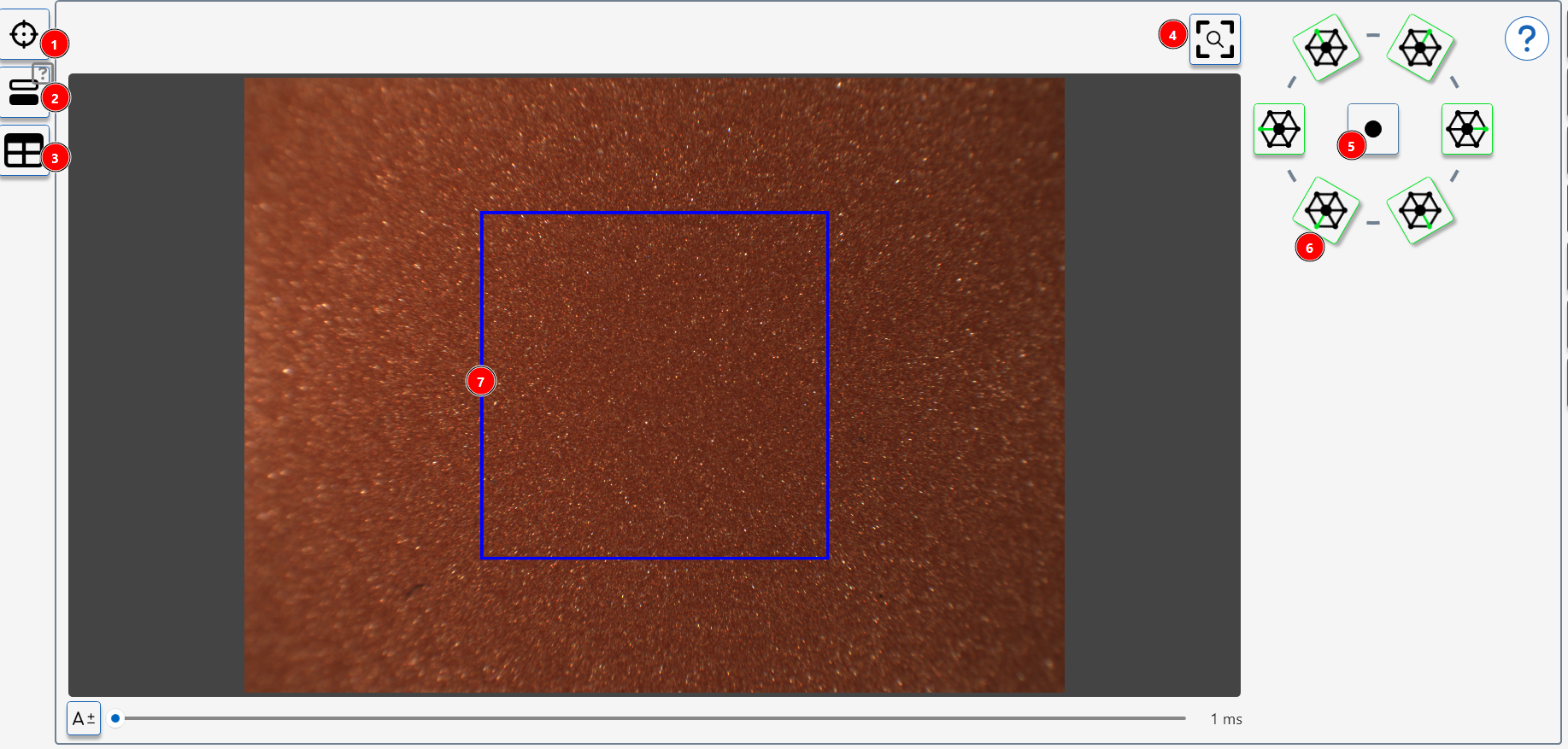
- Take a measurement
- Start calibration Procedure
- Switch to main screen with table
- Recentre camera view
- Switch on 10 degree spot light
- Switch on 45 degree light source(s)
- Standard sparkle measurement area.
Measurement Procedure
- Ensure the sensor is calibrated.
- Press the button (1) to activate the interactive measurement feature.
- Adjust the light sources as required, recommended setting are 45 Degree Light Sources- all illuminated, or single spot light only illuminated.
- Use the auto-exposure button to optimize the camera exposure for the surface's reflectivity.
- Manually adjust exposure if needed using the slider or input box.
- The blue square indicates the measurement area for this module.
- To measure the sparkle and graininess of an identified area on the surface move the sensor until the required area is enclosed by the blue square.
Texture Module
The Rhopoint Aesthetix Texture Module provides objective analysis of the surface characteristics critical to visual perception and quality control for textured surfaces.
Textured surfaces are those with irregular or patterned finishes, differing from smooth or flat surfaces. These textures can be natural or manufactured and include features like ridges, grooves, bumps, or grains that affect the material's tactile and visual properties.
Examples include:
Leather-like Surfaces: Found in automotive interiors and furniture, mimicking natural leather.
Coated Surfaces: Textured paint or powder coated surfaces on metal or plastic, influencing appearance and feel.
Plastic pars: Moulded textures in consumer electronics and automotive components for grip and aesthetics
Textured surfaces are crucial in many industries for their impact on product aesthetics, functionality, and consumer perception, such as automotive, powder coating and leather manufacture, ensuring enhanced quality control, product development, and consistency across global supply chains.
Using Aesthetix, the user can reduce subjective errors associated with visual inspection, ensuring measured surfaces have the required perceived quality and good harmony with adjacent parts.
Measurement Method
RGB colour, gloss, reflectivity, and 3D topography measurements are combined into a single measurement, delivering precise and repeatable results.
The Aesthetix uses utilizes photometric stereo techniques to estimate surface normals and calculate 3D topography, providing a detailed height map of the surface.
A watershed algorithm is then applied to segment the topography into cells, allowing for the analysis of cell size and area.
60° gloss is measured and reported, fully compliant with international norms ASTM D523 & ISO 2813.
RGB colour is measured using 45°:0° geometry and the reported values are calculated using the average RGB pixel value of the area captured by the observer camera.
Reflectance parameters are calculated using the gloss camera & reflectance differences measured using the observer camera.
Texture feature properties (watershed methodology)
Watershed Overview
To separate features on the surface, a so-called “watershed algorithm” is applied to the topographic height map.
A flooding analogy can be used to understand the watershed principle.
The measured topographical map can be treated like a landscape of hills and valleys.
When water is poured into the landscape, and the water level rises, the valleys (which are the local minima of the gradient image) start filling up with water, separating the hills as islands (“features”).
When water from two different valleys meet and merge, a dam (or watershed line) is constructed to prevent merging.
These watershed lines effectively become the boundaries between different regions in the image.
The result is a segmented image where each region is separated by watershed lines, corresponding to different features within the surface.
![Topographical height map]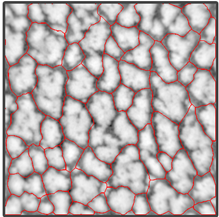
Topographical height map of a surface with watershed analysis applied
Control over how the watershed lines are constructed in Appearance Elements is given in the “Feature Properties” settings.
Adjusting Texture Module User Parameters
Adjusting the Feature Properties (Watershed parameters)
Manual Adjustment of the Feature separation

- Visual Inspection
Start by visually inspecting the height image and the initial segmentation results by using the default settings
(Default: Feature separation: 3px, Feature selection: 70%).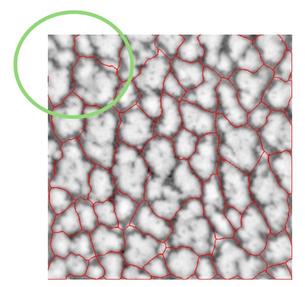
In the image above, the default settings have not segmented the whole map successfully- by visual inspection we can see that some features are not separated. In this example features are separated by low areas (valleys) and represent distinct high areas or hill.
- Adjust Thresholds
Modify the watershed parameters in “Feature properties” and observe the effect on the feature detection.
Adjust Feature properties and test different values, then evaluate their impact on the segmentation.
Feature Separation (Watershed Morphology)
This parameter increases the gap between the found features (hills) by the separation value (number of pixels)
Increasing the amount of Pixels used will separate some touching features, and thus increase the number of detected features (hills).
Feature Selection (Watershed Selection Percentage)
This value from 0% to 100% determines which size of features (hills) are included in the evaluation after separation.
While increasing this number will exclude smaller unwanted features, it should be reduced for smaller shapes.
In the analysis the watershed algorithm has not separated all the features (hills)- the feature separation parameter “Feature selection” should be increased.
Watershed parameter adjustment
To adjust the areas selected by the watershed.
- Click the settings button on the right side menu.
- Click the plus button to expand “Feature properties”.
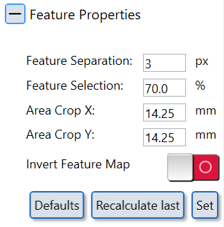
Adjust “Feature Separation” (watershed morphology) and “Feature Selection” (Watershed Selection Percent) parameters.
- Press "Set" button.
- Press "Recalculate last" button.
Increased Feature Separation value will now correctly analyse the shapes.
!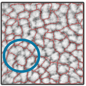 |
!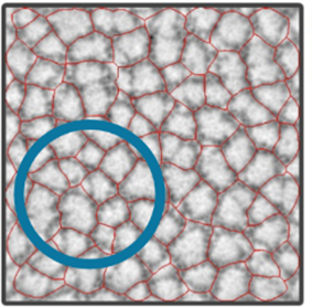 |
|---|---|
| Before | After |
Invert feature map algorithm
Standard textures and Leather are described by hills which are spatially separated by valleys.
Some technical textures, however, form the actual texture by hills (along their maxima).
For these textures, the standard algorithm will not yield a good or none result, in which case the algorithm has to be “inverted”.
When this happens, please use the “Invert Feature Map” setting, set and recalculate.
Example: the measurement of a technical laser texture does not yield any reasonable results, no matter what is set up in feature selection.
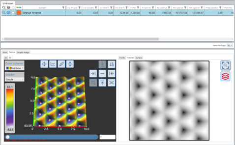
After selection of “Invert Feature Map” and setting appropriate values, the results become reasonable.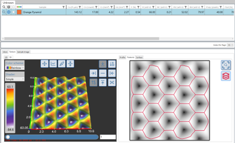
Cutting the area of interest
For some applications it might be advisable that the area of interest is cut to a smaller or even larger region than the default (10.00mmx10.00mm), e.g., for steel or metallized surfaces.
This helpful in those cases were there are damages or over illumination due to material albedo at the edges.
In this case, you cut to a more specific region, defining an area by width and height (X and Y) distance, around the centre point of the image (0/0).
For example, Standard setup 10.00mmx10.00mm, from centre point 5.00mm to the left and to the right, as well as 5.00mm up and 5.00mm down.
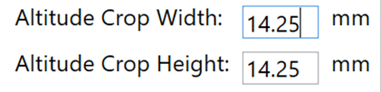
Cut to 10x10, or 5mm in all directions: enter 10mm Width and Height, “Set” and “Recalculate last”.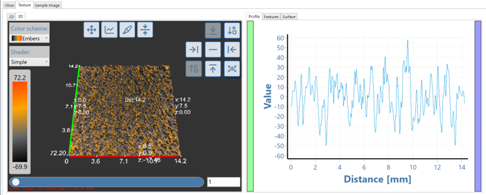
Texture Module Parameters
| Index | Name / Title | Unit | Description |
|---|---|---|---|
| 60° | 60° Gloss | GU | Conventional 60° gloss value of the textured area, indicating overall specular reflectance level. |
| Sa Rough | Areal Surface Roughness | p‑µm | Average height variation over the measured area using unfiltered topographical data, expressed in perceived microns. |
| Ca | Cell Altitude | p‑µm | Average height of texture “cells” (features) relative to the local mean plane. |
| Cn | Cell Number | – | Total number of detected texture cells within the analysed area. |
| Cs | Mean Cell Size | p‑µm | Average lateral size of the detected texture cells. |
| CsMin | Minimum Cell Size | p‑µm | Smallest detected cell size within the measurement area. |
| CsMax | Maximum Cell Size | p‑µm | Largest detected cell size within the measurement area. |
| CsDev | Cell Size Standard Deviation | p‑µm | Variation (spread) of cell sizes, indicating how uniform the texture features are. |
| Hs | Hill Size | p‑µm | Typical size of raised “hill” features on the surface. |
| F | Fill Factor | – | Fraction of the area occupied by detected texture cells or hills. |
| R | Reflectivity | – | Average reflectivity level of the textured surface region. |
| RC | Reflective Contrast | – | Difference in reflectivity between texture features and surrounding areas. |
| RV | Reflectivity in Valleys | – | Reflectivity associated with valley (low) regions of the texture. |
| RH | Reflectivity on Hills | – | Reflectivity associated with hill (high) regions of the texture. |
| Fsep | Feature Separation | µm | Records the user setting for Feature Seperation parameter |
| Fsel | Feature Selecttion | %tage | Records the user setting for Feature Selection parameter analysis. |
| FThld | Feature Threshold | -1 to +1 | Records the user setting for Feature Threshold parameter analysis. |
| R (RGB) | Red RGB Colour | Intensity (0–255) | Average red-channel surface colour within the textured area. |
| G (RGB) | Green RGB Colour | Intensity (0–255) | Average green-channel surface colour within the textured area. |
| B (RGB) | Blue RGB Colour | Intensity (0–255) | Average blue-channel surface colour within the textured area. |
Topographical Graph Scale- Perceived Microns [pµm]
Interpreting Surface Texture Results
How Does Aesthetix Measure Surface Texture?
The Aesthetix uses advanced optical and computational techniques to measure surface texture. It employs photometric stereo imaging to estimate surface normals and create detailed 3D topographical maps. These maps represent the height variations across the surface, allowing precise analysis of texture features. The system uses a watershed algorithm to segment the surface into distinct cells (hills and valleys), enabling the quantification of structural features such as height, size, and distribution.
Key steps in the measurement process:
- Image Capture: The system captures multiple images under different lighting conditions to calculate surface normals.
- 3D Topography: A height map is generated to represent the vertical variations of the surface.
- Segmentation: The watershed algorithm separates features into cells, identifying hills, valleys, and their boundaries.
- Analysis: Metrics such as roughness, cell amplitude, cell size, and reflectivity are calculated from the segmented data.
Measurements Provided by Aesthetix for Surface Texture and Reflectivity
The Aesthetix provides a comprehensive set of metrics to describe surface texture and reflectivity:
Texture Metrics
- Sa (Roughness): Standard deviation of amplitude (height variations) across the surface.
- Ca (Cell Amplitude): Average height difference between hills and valleys, measured in perceived microns (p-µm).
- Cn (Cell Number): Total number of distinct cells or features within the measurement area.
- Cs (Cell Size): Includes mean, minimum, maximum, and standard deviation of cell sizes (mm²).
- Hs (Hill Size): Average cross-sectional area of elevated features (mm²).
Reflectivity Metrics
- R (Reflectivity): Average reflectivity value of the surface in arbitrary units.
- RC (Reflective Contrast): Difference in reflectivity between hills and valleys.
- RH/RV: Reflectivity values specific to hills and valleys.
Comparison and Application
- Use Sa for general roughness analysis when evaluating overall surface smoothness.
- Select Ca for assessing depth or relief of textures that influence tactile or visual perception.
- Use Cn and Cs for understanding feature density and uniformity, critical for textured coatings or molded parts.
- Reflectivity metrics like RC are ideal for determining how texture impacts visual contrast or glossiness.
Choose metrics based on your application:
- For functional surfaces requiring uniformity (e.g., automotive interiors), focus on Cn, Cs, and RC.
- For aesthetic surfaces where depth or relief matters (e.g., leather-like finishes), prioritize Ca and Sa.
Visualizing Surface Texture Using Appearance Elements
The Rhopoint Appearance Elements software enables users to visualize and analyze surface texture in detail. Follow these steps to effectively examine the surface's 3D structure, depth, and features:
- Open the 3D View in the Left Window:
- Navigate to the left-hand panel of the software and select the "3D View" tab.
- The surface's topographical map will be displayed as a 3D model, color-coded to represent height variations.
- Use the mouse or navigation tools to rotate, zoom, and pan the 3D map for a comprehensive view of the surface.
- Use the Profile Tool in the Map Window:
- Switch to the "Map View" in the central window to view a 2D representation of the surface's height map.
- Select the "Profile Tool" (typically represented by a line icon).
- Click and drag across the map to draw a line indicating your region of interest. This line will serve as a cross-section for further analysis.
- Open the Profile View in the Right Window:
- Navigate to the right-hand panel and select the "Profile View" tab.
- The profile view will display a cross-sectional graph of the surface along the drawn line, showing height variations in perceived microns (p-µm).
- Peaks represent hills or elevated areas, while valleys indicate depressions or lower regions on the surface.
- Analyze Cell Size Using the Features Window:
- Open the "Features Window" in the right-hand panel.
- This window provides detailed information about identified surface features, including hills, valleys, and cells segmented by a watershed algorithm.
- Metrics such as cell size (mean, minimum, maximum), cell amplitude (height differences), and cell number are displayed. These values help evaluate texture uniformity, density, and depth.
- Adjust Visualization Settings:
- Modify watershed parameters (e.g., feature separation or selection) in the settings menu to refine feature detection and segmentation.
- Use color scales or visual overlays to enhance specific areas of interest.
By combining these tools, you can gain a detailed understanding of your surface's texture, including its depth, uniformity, and structural features. This visualization process is essential for quality control, product development, and ensuring consistency across manufacturing processes.
Adjusting Surface Texture or Reflectivity
To modify surface texture:
- Surface Preparation:
- Sanding or polishing can reduce roughness (Sa) and improve smoothness.
- Texturing processes like embossing or chemical etching can enhance relief (Ca) or create specific patterns.
- Tool Design or Wear:
- Cell size is fixed during tool design and manufacture, Reflectivity and cell depth can be effected by tool wear. (Cn, Cs) and reflectivity (R, RC).
By selecting appropriate processes based on Aesthetix measurements, you can achieve desired aesthetic or functional outcomes while maintaining consistency across production batches.
Polishing Quality Module
The Polishing Quality module evaluates how well a high-gloss surface has been polished by simultaneously quantifying gloss, haze, sharpness/DOI and polishing defects such as scratches, swirls and holograms. It turns what would normally be a subjective visual judgement into objective, repeatable numbers that closely reflect how clean, sharp and defect‑free the surface appears to the human eye.
Purpose of this module
- Optimise and control polishing processes by measuring the presence and severity of fine scratches, swirls and holograms together with gloss, haze and sharpness.
- Provide perception‑aligned metrics that allow OEMs, body shops and suppliers to agree clear pass/fail limits for polishing quality, reducing rework and disputes.
Where this module can be used
- High‑gloss automotive exterior and interior components, including clearcoats, spot repairs, piano black trims and high-end refinish work.
- Premium consumer goods, furniture, glass and plastic parts where ultra‑smooth, scratch‑free finishes are critical for perceived quality and brand image.
What this module measures
- Gloss, haze (including LogH / LogH C) and sharpness/DOI to characterise overall reflectivity, depth of finish and image clarity of the polished surface.
- Scratch and polishing defect metrics such as scratch length, scratch count, total area and visibility giving a detailed map of swirl marks and micro‑scratches.
How to use this module
- In Rhopoint Appearance Elements, select the Polishing Quality module, choose the correct adaptor or stand for the part geometry, and calibrate on the supplied reference tile as recommended.
- Position the Aesthetix sensor over the area of interest (for example a polished panel or spot repair), trigger one or more measurements, then save the numerical results and images into the relevant job, batch or template.
How to interpret the results
- Use gloss, haze and sharpness/DOI values to confirm that the overall level of mirror‑like finish meets specification, and to detect over‑ or under‑polishing with the haze parameters.
- Review scratch length, area, count and visibility values (and corresponding images) to decide whether swirls, holograms and micro‑scratches are below acceptable thresholds, and to compare different polishing compounds, pads or process steps.
Measuring Polish Quality
Select a measurement mode
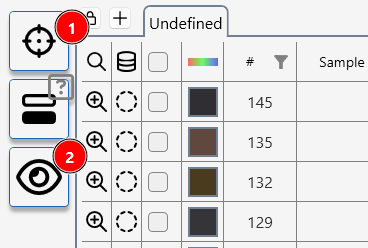
To measure polishing quality with default or last used parameters, press (1) a measurement will be made results will be added to the data table.
To adjust parameters before starting a measurement, click the interactive measurement icon (2).
Surface Preview
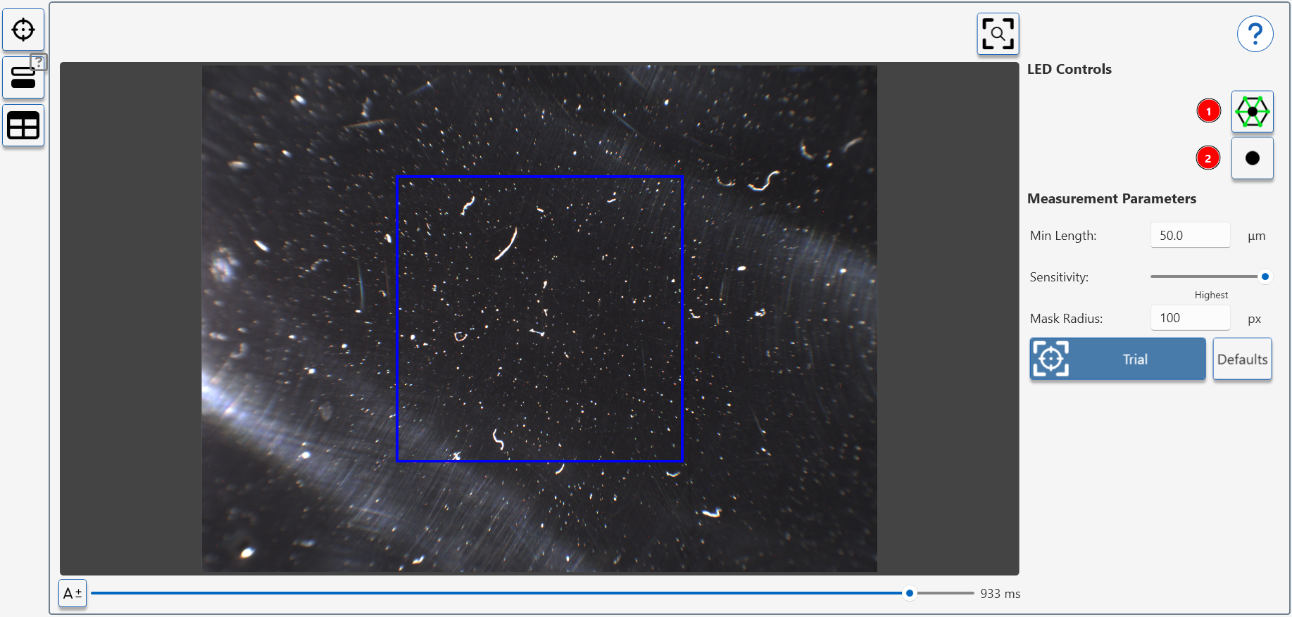
The surface preview is used to position the sample over an area of interest. The 45 degree ring lights show surface damage and marks.
Analysis for polishing marks is made using the 10 degree spot light- press (2) to activate this.
Analysis Preview
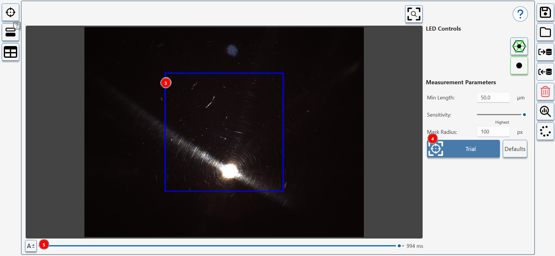
A blue box (1) shows the measurement area.
Press (2) to take a a trial measurement.
Adjust settings (3) to change camera exposure settings (changing exposure in this view does not effect measurement).
Measurement Preview
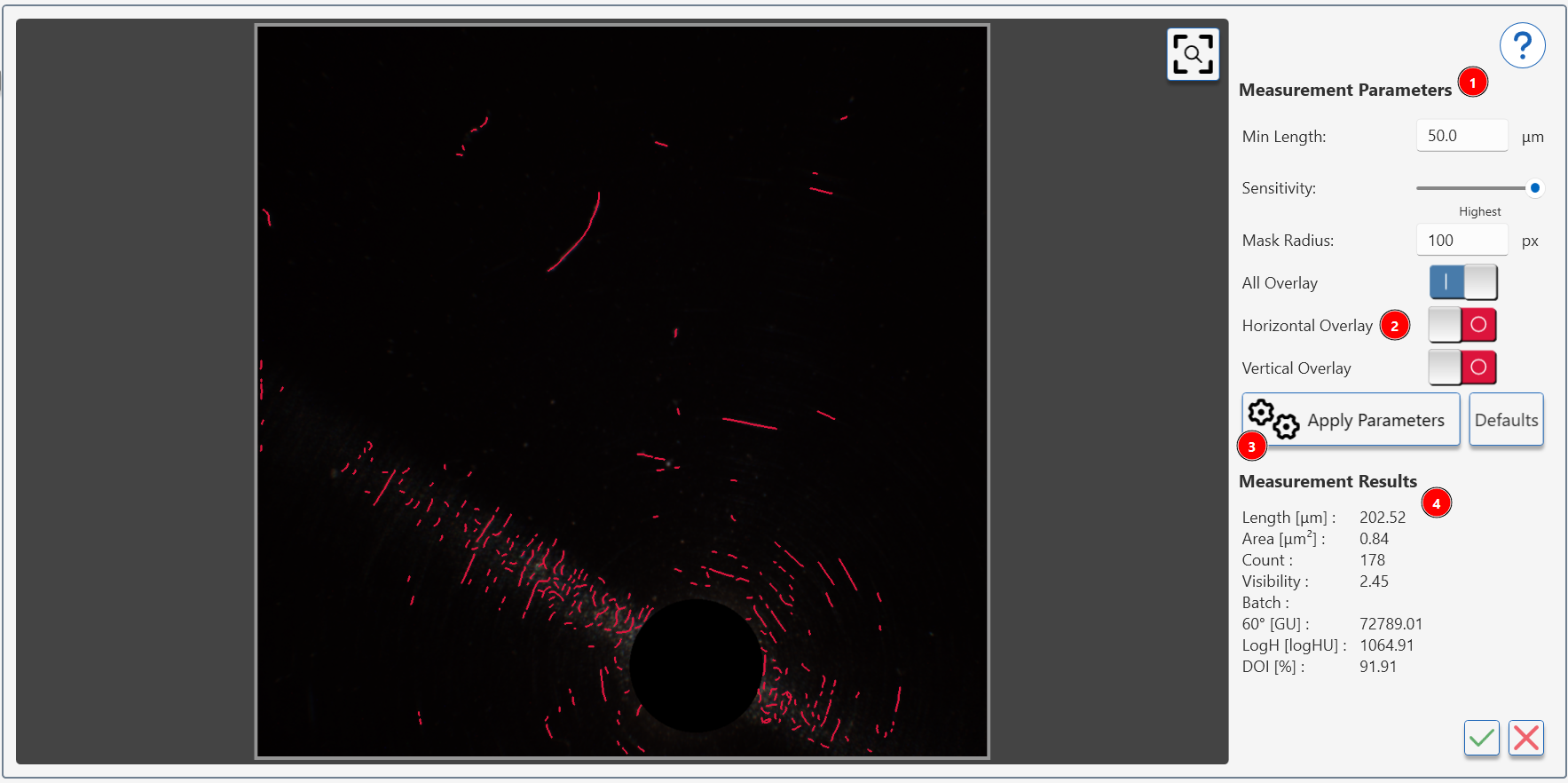
When a preview measurement has been completed the results are shown in a preview window.
The left image shows the identified damage on the surface, adjusting the measurement parameters (1) will change the amount of detected damage.
How to adjust Polishing Quality Parameters
The overlay control (2) highlight 'horizontal', 'vertical' or 'all' scratches. These values are recorded separately in the measurement data and can be used to detect directional damage in the surface.
To recalculate the measurement results (4) adjust the parameters (1) and press apply parameters icon (3).
Complete or restart measurement
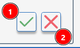
To complete the measurement process, press the tick icon (1)- the trial measurement values will be transferred to the data table.
To restart the process press the cancel icon (2).
Review measurement results
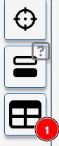
To review measurements in the table, press the table icon (1).
Adjusting Polishing Quality Parameters
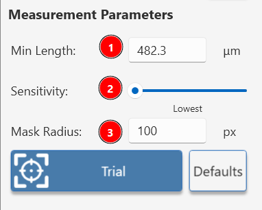
1. Minimum Length
- Purpose: Sets the smallest size of defects to be included in the analysis, measured in microns.
- How It Works:
- Larger values exclude smaller defects, focusing on more significant imperfections.
- Smaller values include finer defects but may increase detection of irrelevant marks.
- Adjustment Steps:
- Begin with a moderate value based on your quality standards (Default is 100 microns).
- Decrease the value if you need to detect shorter defects.
- Increase the value to focus only on larger imperfections.
- Adjust based on the typical size of defects relevant to your product quality criteria.
2. Sensitivity
- Purpose: Controls the threshold for detecting linear defects based on their visibility (contrast against the background).
- Options: Lowest, Low, Moderate, High, Highest
- How It Works:
- Higher sensitivity detects more subtle defects but may include false positives.
- Lower sensitivity focuses on more prominent defects, potentially missing subtle ones.
- Adjustment Steps:
- Start with "Lowest" sensitivity.
- If important defects are missed, increase the sensitivity.
3. Mask Radius
- Purpose: Excludes the direct reflection of the high-intensity spot from the analysis.
- The default radius removes the spot reflection in smooth mirror like surface.
- Increase the radius if surface haze or polishing marks are increasing the reflected spot size and interfering with defect detection.
Polishing Quality Parameters
| Index | Name / Title | Unit | Description |
|---|---|---|---|
| 60° | 60° Gloss | GU | Conventional 60° gloss value indicating overall specular reflectance of the polished area. |
| S | Sharpness | % | Measures image sharpness/clarity in the reflected image, related to DOI; higher values mean crisper reflections. |
| MC Haze | Michelson Haze | HU | Quantifies haze as low-contrast veiling around reflections that reduces clarity on polished surfaces. |
| LogH C | LogHaze Compensated | logHU | Compensated LogH value that corrects for gloss level, aligning more closely with visual perception of haze. |
| VisH-Out | Visual Haze Outdoors | VHU | Perception-based haze index modelling how haze appears under outdoor/daylight conditions. |
| VisH-In | Visual Haze Indoors | VHU | Perception-based haze index modelling how haze appears under indoor/controlled lighting. |
| DOI | Distinctness of Image | % | Describes how clearly objects are reflected in the surface; low DOI indicates milky or blurred reflections. |
| Min Length | Minimum Detection Length | µm | Parameter which determines the minimum length of detected scratches. |
| Sensitivity | Sensitivity of Detection | – | Parameter which controls the sesnistivity of the scratch detection algorithm. |
| Mask Radius | 10° Spot Covering Mask Area | Pixel | Parameter which sets the radius of the analysis mask used around the 10° spot when detecting scratches. |
| Length | Average Scratch Length | µm | Average length of all detected scratches in the measurement area. |
| Length V | Average Scratch Lengh Vertical | µm | Average length of scratches predominantly oriented in the vertical direction. |
| Length H | Average Scratch Lengh Horizontal | µm | Average total length of scratches predominantly oriented in the horizontal direction. |
| Area | Total Scratched Area | µm² | Combined area covered by all detected scratches. |
| Area V | Scratched Area Vertical | µm² | Total area of vertically oriented scratches. |
| Area H | Scratched Area Horizontal | µm² | Total area of horizontally oriented scratches. |
| Count | Total Scratches | – | Total number of scratches detected in the analysed area. |
| Count V | Scratches Vertical | – | Number of vertically oriented scratches. |
| Count H | Scratches Horizontal | – | Number of horizontally oriented scratches. |
| Visibility | Scratch Visibility Average | AU* | Average perceived visibility of all detected scratches. |
| Visibility V | Scratch Visibility Vertical | AU* | Perceived visibility of vertically oriented scratches. |
| Visibility H | Scratch Visibility Horizontal | AU* | Perceived visibility of horizontally oriented scratches. |
| R (RGB) | Red Channel Colour | Intensity (0–255) | Average red-channel surface colour in the analysed area. |
| G (RGB) | Green Channel Colour | Intensity (0–255) | Average green-channel surface colour in the analysed area. |
| B (RGB) | Blue Channel Colour | Intensity (0–255) | Average blue-channel surface colour in the analysed area. |
*AU = arbitrary (instrument) units.
Interpreting Polishing Quality Results
How Does Aesthetix Measure Polishing Quality (Scratches, Swirls, and Holograms)?
The Aesthetix evaluates polishing quality by using high-resolution imaging and advanced algorithms to detect and quantify surface defects such as scratches, swirls, and holograms. These imperfections are identified based on their unique visual characteristics under specific lighting conditions.
Measurement Process:
- Directional Illumination: The Aesthetix uses multiple light sources, including a 10° point light and a 45° ring light, to illuminate the surface. These lighting setups enhance the visibility of defects like scratches, swirls, and holograms.
- High-Resolution Imaging: A camera captures detailed images of the illuminated surface. Scratches appear as linear features, swirls as concentric circular patterns, and holograms as elongated streaks starting from the light source.
- Image Analysis: The system applies image segmentation algorithms to isolate and quantify these defects. Metrics such as defect length, width, density, and orientation are calculated.
This approach ensures precise detection of polishing defects that are often difficult to identify under standard inspection conditions.
Additional Measurements Provided by Aesthetix
In addition to detecting scratches, swirls, and holograms, the Aesthetix provides several advanced metrics to further analyse surface quality:
- Sharpness:
- Measures the clarity and definition of edges in reflected images.
- Higher sharpness values (measured in Sharpness Units [SU]) indicate clearer reflections with well-defined edges.
- Useful for assessing overall surface quality and how well the surface reflects fine details.
- Distinctness of Image (DOI):
- Evaluates the overall clarity of reflected images.
- Higher DOI values indicate less distortion in reflections, making it ideal for applications requiring smooth finishes (e.g., automotive coatings).
- LogHaze C:
- Quantifies technical haze caused by light scattering around a specular reflection.
- Important for identifying micro-textures or contaminants that reduce clarity.
- Visual Haze Outdoor (VHout):
- Adjusts haze measurements to match human perception under outdoor lighting conditions.
- Critical for applications where products are viewed in bright sunlight or high-intensity lighting environments.
Comparison and Application:
- Use Sharpness for high-gloss surfaces where edge clarity is critical (e.g., automotive finishes or polished metals).
- Choose DOI when assessing the overall distinctness of reflections is more important than edge sharpness.
- Select LogHaze C for technical analysis of haze caused by micro-textures or contaminants.
- Opt for Visual Haze Outdoor when evaluating surfaces intended for outdoor use, ensuring defects like holograms or haze are not visible under sunlight.
Each metric provides unique insights into surface quality; selecting the right one depends on your specific application requirements.
Visualising Polishing Quality Using Appearance Elements
The Rhopoint Appearance Elements software enables detailed visualisation of polishing quality:
- Open Defect View:
- Navigate to the "Defect View" tab in the software.
- Use directional lighting options (e.g., 10° point light) to highlight surface imperfections.
- Analyse Defects:
- Scratches appear as linear features in the captured images.
- Swirls are displayed as circular patterns, while holograms appear as elongated streaks.
- Colour-coded overlays can be applied to distinguish between defect types.
- Visualise Advanced Metrics:
- Access additional views for Sharpness, DOI, LogHaze C, and Visual Haze Outdoor.
- Compare these metrics side-by-side with defect visualisations to correlate numerical values with observed imperfections.
- Quantitative Analysis:
- View metrics such as scratch density, swirl intensity, sharpness units (SU), DOI values, and haze levels in the results panel.
- Compare multiple samples side-by-side for consistency checks.
- Export Results:
- Save annotated images and data for reporting or further analysis.
Improving Polishing Quality (Reducing Visibility of Scratches, Swirls, and Holograms)
To improve polishing quality and reduce visible defects:
- Optimise Polishing Techniques:
- Use finer abrasives or polishing compounds to minimise scratches.
- Avoid excessive pressure during rotary polishing to reduce swirl marks.
- Use dual-action polishers instead of rotary tools to prevent holograms.
- Control Environmental Factors:
- Ensure a clean workspace to avoid introducing dust or debris during polishing.
- Maintain consistent temperature and humidity to optimise compound performance.
- Use High-Quality Materials:
- Select premium polishing pads and compounds designed for specific surface types.
- Ensure compatibility between pads, compounds, and coatings.
- Inspect Regularly During Polishing:
- Periodically check surfaces under directional lighting to identify defects early.
- Adjust techniques or materials as needed based on real-time feedback.
- Apply Protective Coatings:
- Use sealants or ceramic coatings after polishing to protect against future scratches or defects.
By leveraging precise measurements from Aesthetix alongside these improvement strategies, manufacturers can achieve consistently high-quality finishes with minimal visible imperfections while ensuring alignment with human perception under various lighting conditions.
Linear Scratch Module
The Linear Scratch module uses the 45° circumferential light source and observer camera to detect and quantify linear and small-area defects—such as scratches, dents, streaks and contamination—that are visible under normal viewing conditions, for example in a laboratory light booth or typical office lighting. It turns what would normally be a subjective visual check under standard room lighting into clear numerical indicators that can be trended, compared and specified.
Purpose of this module
- Identify and measure linear and local defects that reduce perceived surface quality in everyday viewing environments, not just under extreme or artificial inspection lighting.
- Provide process feedback so you can compare cleaning, coating and handling steps, and set objective pass/fail limits for scratches, dents, streaks and visible contamination.
How defects are detected
- The module uses a 45° circumferential light source to illuminate the surface uniformly from all directions at 45°, closely mimicking common overhead and light‑booth conditions while enhancing the visibility of defects.
- A camera observes the same area and captures high‑resolution images in which scratches, dents, streaks and contaminants appear as local changes in brightness, relative to the surrounding surface.
- Image‑processing algorithms then separate these defect features from the normal background appearance, classify them by type and geometry, and calculate parameters such as length, area, count and visibility.
Directional categorisation: horizontal and vertical scratches
Detected linear features are further analysed by their orientation on the surface and automatically classified as predominantly horizontal or vertical scratches.
By comparing the total length, area and count of horizontal versus vertical scratches, the Aesthetix can reveal inhomogeneity or directional damage, for example abrasion caused by a process step that acts mainly in one direction (such as machine polishing, wiping or conveyor contact).
This directional information helps users diagnose root causes more quickly, adjust process settings (tool paths, wiping direction, handling fixtures) and verify that corrective actions have reduced directional scratching rather than simply changing its orientation.
Role of sensitivity
- A Sensitivity control adjusts how strongly the detection algorithm responds to subtle defect features in the images.
- At low sensitivity, only the most obvious scratches and defects are reported, corresponding to marks that are clearly visible under normal office or light‑booth conditions.
- At medium sensitivity, the module reveals finer streaks, lighter scratches and small contamination spots that may be noticed by trained inspectors or under slightly more critical viewing.
- At the highest sensitivity, all visible linear and local features are highlighted, including faint defects that may only be noticed under very critical inspection, while still being evaluated within a normal‑lighting context.
What this module measures
- Length parameters (total, vertical and horizontal) describe how extensive linear defects such as scratches and streaks are, and whether they are predominantly oriented in one direction.
- Area parameters quantify how much of the measured region is covered by detected defects (scratches, dents, contamination), again split into total, vertical and horizontal components where applicable.
- Count parameters report how many individual defect features are present for each orientation or class, giving a simple defect density measure.
- Visibility parameters express how noticeable these defects are under typical viewing conditions, combining their size, brightness and contrast into perception‑based values.
How to use this module in practice
- Use lower sensitivity settings and the visibility parameters to set realistic acceptance criteria that reflect what customers and end‑users see in laboratory booths, offices or showrooms.
- Increase sensitivity when you need to diagnose underlying quality issues, compare alternative process steps, or ensure that a premium surface remains visually clean and uniform under more critical inspection.
- Trend defect metrics over time or between batches to confirm that surface preparation, coating, polishing and handling processes are stable, and that any changes in materials or equipment do not introduce new visible defects.
System Requirements
Before installing, check the requirements for the host PC.
Recommended System Requirements
- OS: Windows 11 (Windows 10 support ends October 2025)
- Memory: 16 GB
- CPU: x64 (x86 and ARM are not supported)
- Port: USB 3.0 USB-C or Thunderbolt
- Screen Resolution: 1920 x 1080
Minimum System Requirements
- OS: Windows 11 (Windows 10 support ends October 2025)
- Memory: 8 GB
- CPU: x64 (x86 and ARM are not supported)
- Port: USB 3.0 USB-C or Thunderbolt
- Screen Resolution: 1440 x 900
Measuring Linear Scratches
Select a measurment mode
To measure polishing quality with default or last used parameters, press (1) a measurment will be made and the results will be added to the data table.
To adjust parameters befoe starting a measurement, click the interactive measurement icon (2).
Analysis Preview
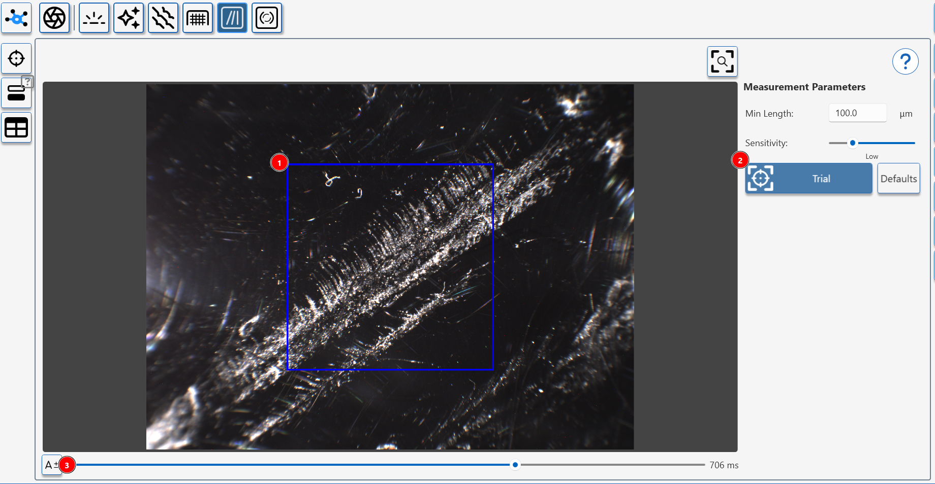
The analysis preview shows a live view from the observer camera.
A blue box (1) shows the measurement area.
Adjust settings (3) to change camera exposure settings (changing exposure in this view does not effect measurement).
Press (2) to take a a trial measurement.
Measurement Preview
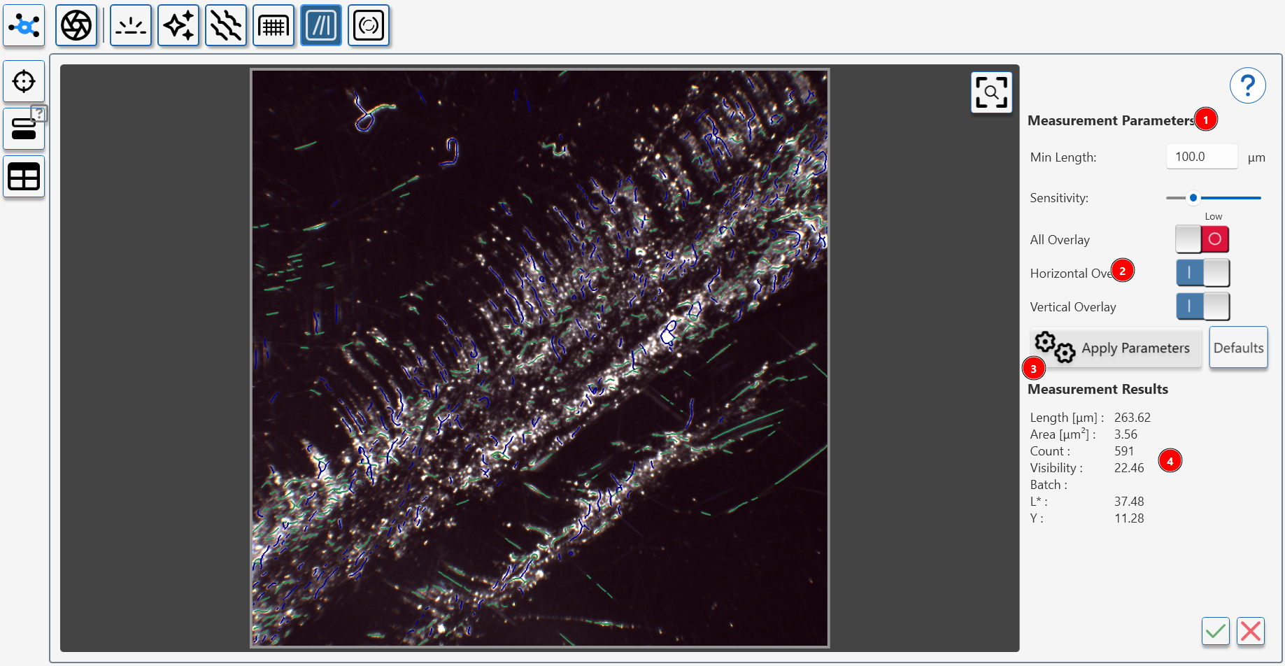
When a preview measurment has been completed the results are shown in a preview window.
The left image shows the identified damage on the surface, adjusting the measurement parameters (1) will change the amount of detected damage.
How to adjust Polishing Quality Parameters
The overlay control (2) highlight 'horizontal', 'vertical' or 'all' scratches. These values are recorded seperately in the measurement data and can be used to detect directional damage in the surface.
To recalculate the measurement results (4) adjust the parameters (1) and press apply parameters icon (3).
Complete or restart measurement
To complete the measurement process, press the tick icon (1)- the trial measurement values will be transfered to the data table.
To restart the process press the cancel icon (2).
Review measurement results
To review measurments in the table, press the table icon (1).
Linear Scratch Parameters
| Index | Name / Title | Unit | Description |
|---|---|---|---|
| 60° | 60° Gloss | GU | Conventional 60° gloss value indicating overall specular reflectance of the polished area. |
| Min Length | Minimum Detection Length | µm | Parameter which determines the minimum length of detected scratches. |
| Sensitivity | Sensitivity of Detection | – | Parameter which controls the sesnistivity of the scratch detection algorithm. |
| Mask Radius | 10° Spot Covering Mask Area | Pixel | Parameter which sets the radius of the analysis mask used around the 10° spot when detecting scratches. |
| Length | Average Scratch Length | µm | Average length of all detected scratches in the measurement area. |
| Length V | Average Scratch Lengh Vertical | µm | Average length of scratches predominantly oriented in the vertical direction. |
| Length H | Average Scratch Lengh Horizontal | µm | Average total length of scratches predominantly oriented in the horizontal direction. |
| Area | Total Scratched Area | µm² | Combined area covered by all detected scratches. |
| Area V | Scratched Area Vertical | µm² | Total area of vertically oriented scratches. |
| Area H | Scratched Area Horizontal | µm² | Total area of horizontally oriented scratches. |
| Count | Total Scratches | – | Total number of scratches detected in the analysed area. |
| Count V | Scratches Vertical | – | Number of vertically oriented scratches. |
| Count H | Scratches Horizontal | – | Number of horizontally oriented scratches. |
| Visibility | Scratch Visibility Average | AU* | Average perceived visibility of all detected scratches. |
| Visibility V | Scratch Visibility Vertical | AU* | Perceived visibility of vertically oriented scratches. |
| Visibility H | Scratch Visibility Horizontal | AU* | Perceived visibility of horizontally oriented scratches. |
| R (RGB) | Red Channel Colour | Intensity (0–255) | Average red-channel surface colour in the analysed area. |
| G (RGB) | Green Channel Colour | Intensity (0–255) | Average green-channel surface colour in the analysed area. |
| B (RGB) | Blue Channel Colour | Intensity (0–255) | Average blue-channel surface colour in the analysed area. |
*AU = arbitrary (instrument) units.
Cross-cut Module
Cross-cut Module
Aesthetix Cross-cut Module replaces the subjective visual analysis of cross-cut panels with reproducible imaging measurement.
In the paint and coatings industry, adhesion is a critical property that determines the durability and performance of a coating under various conditions.
In the paint and coatings industry, adhesion is a critical property that determines the durability and performance of a coating under various conditions.
The Cross-cut Test, standardized by ISO (International Organization for Standardization) under ISO 2409, is a widely recognized method for evaluating the adhesion of a coating to a substrate.
Why Cross-cut Testing is Important
Adhesion as a Key Quality Indicator
Coatings are applied to protect surfaces from environmental damage, corrosion, or wear, and to enhance aesthetics. A coating's ability to adhere strongly to a substrate ensures it performs its intended function over time without peeling, flaking, or detaching.
Reliability Across Industries
Cross-cut testing is used globally to ensure coatings meet consistent quality and performance standards. It helps manufacturers, contractors, and end-users to validate product reliability, regardless of the substrate type or environmental conditions.
Ease and Precision
The test involves making a grid of cuts (cross-cuts) through the coating down to the substrate using a specialized cutting tool. After the grid is created, adhesive tape is applied and removed to assess the coating's adhesion based on the extent of detachment or flaking observed in the cut areas. The results are graded on a numerical scale, making it a simple yet precise evaluation method.
Standardized Benchmarking
By following the ISO 2409 standard, the test provides a clear benchmark for comparing coating performance. This helps in quality control, product development, and ensuring compliance with industry regulations.
Cross-cut Testing with Aesthetix
The Aesthetix device leverages the principles of the ISO Cross-cut Test to provide accurate and repeatable measurements of cross-cuts, not being subject to daily form.
With Aesthetix, users can efficiently and neutrally assess the durability of their coatings, ensuring they meet both performance expectations and industry standards. This empowers paint and coating professionals to achieve superior product performance and durability.
Cross-cut Properties
The standard method for ISO 2409 proposes to cut six horizontal and six vertical lines.
The Default setting for Appearance Elements is to use this setup with a cut spacing of 2.0 mm, a cut thickness of 0.2mm and a detection threshold of 10%.

Cut Spacing
Cut Spacing (also called line spacing) is the distance between the centers of nearby cut lines.
Cut Thickness
Cut Thickness is how wide each cut line is.
Cut Detection Threshold
Cut Detection Threshold controls how the system tells the difference between areas with coating and areas where the
coating has been removed. The system starts with an automatic guess based on image brightness.
Purpose:
This setting helps fine-tune the system's guess so it better separates coated from uncoated areas. It's especially
useful near the edges where the coating may only be partly removed.
- Raise the threshold to include more subtle changes—this helps catch areas where the coating was lightly removed.
- Lower the threshold to ignore faint signals or small amounts of leftover coating—this helps avoid marking coated areas
as removed.
When to adjust:
Adjust the Cut Detection Threshold if the automatic setting makes mistakes, such as:
- Marking coated areas as removed, or
- Missing areas where the coating was actually removed.
Make small changes and check the results to get the best separation between coated and uncoated regions.
Manual Measurement Method
After setting the properties of the cross-cut detection, the preview will display the cross-cut grid.

Please arrange the grid and the cross-cut image as close as possible, as only a matching overlay would ensure a perfect result. If you see that your grid does not match, please modify the properties accordingly.
Ideal results should look like as in the images below; note that the images show detected remaining coating in green overlay colour:


If you are experiencing issues with the selection of remaining coating, please adjust the Cut Detection Threshold until the resulting overlay is covering the area correctly.
Testing Coatings with Low Absorption Against the Substrate
For samples having a brighter coating compared to the substrate, you might be experiencing issues.
In this case, it might help to use the “Invert Map” setting, to differentiate the cross-cut by inverting the image and then performing the analysis.
How to Measure with Cross Cut Module
How to measure Cross-cut Adhesion
Activate Interactive Measurement
- Press the interactive measurement button.
- Press the interactive measurement button.
Optimize Camera Exposure
- Use the Auto-Exposure button (1) to optimise the camera exposure for the surface's reflectivity.
- If necessary, manually adjust the exposure using the slider. (2).
Choose Automatic or Manual Mode (1)
In auto mode AE detects the cuts, draws the virtual grid and calculates the amount of removed coating.
For irregular grids or tricky applications, the user can use manual mode to select the corners of the cross cut grid.
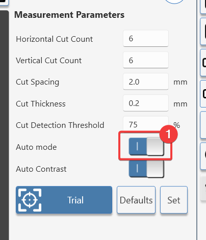
Cross Cut Adhesion Auto Mode
Automatic mode uses image analysis to automatically detect the cuts in the grid and evaluate adhesion with consistent, repeatable results.
Manual mode in the Cross-cut Adhesion module lets the user interactively align the grid and fine‑tune detection settings for difficult materials, such as low-contrast coatings or uneven cross-cut grids.
Activate Interactive Measurement
- In the crosscut module, press the interactive measurement button.
- In the crosscut module, press the interactive measurement button.
Optimize Camera Exposure
Place the instrument on the cross cut test- a clear live image of the surface should be visible.
To adjust the image;
Use the Auto-Exposure button (1) to optimise the camera exposure for the surface's reflectivity.
If necessary, manually adjust the exposure using the slider. (2).
Choose Automatic mode (1)
- Check the Auto mode icon is in the on position (1).
- Choose test parameters
Set grid size (1) and cut parameters to match the test panel (2).
Press the set button (3) to redraw the red guide box (4).
Move the instrument so the guide box (4) is positioned outside the test grid.
Press (5) to start a trial measurement.

- Testing on white or light colours
The default setup detects cut lines that are lighter than the background.
When testing light colours the lines can be darker than the background.
If cut lines are darker that the background colour;
- Switch off auto contrast (1) and select invert image (2)
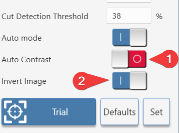
6. Finetuning the detected paint area
The cut detection threshold can be adjusted to;
- Finetune a measurement so edges are more accurately defined.
- Isolate a certain colour of remaining material, for example when determining intercoat adhesion.
- Adjusting the cut detection threshold
Click on/off the found overlay (1).
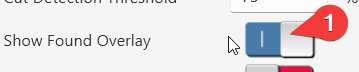
The green overlay should match the area of undamaged coating.
Increasing the threshold (1) makes the detection algorithm more sensitive.
Decreasing the threshold (1) makes it less sensitive.
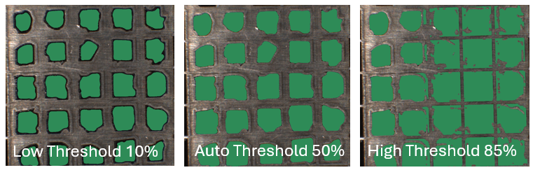
When the found ovelay matches the undamaged pain area;
- Click the accept measurement button (1) to include it in the table.
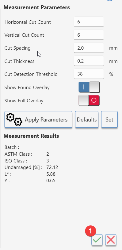
Cross Cut Adhesion Manual Mode
Manual mode in the Cross-cut Adhesion module lets the user interactively align the grid and fine‑tune detection settings for difficult materials, such as low-contrast coatings or uneven cross-cut grids.
Activate Interactive Measurement
- In the crosscut module, press the interactive measurement button.
- In the crosscut module, press the interactive measurement button.
Optimize Camera Exposure
Place the instrument on the cross cut test- a clear live image of the surface should be visible.
To adjust the image;
Use the Auto-Exposure button (1) to optimise the camera exposure for the surface's reflectivity.
If necessary, manually adjust the exposure using the slider. (2).
Choose Automatic mode (1)
- Check the Auto mode icon is in the off position (1).
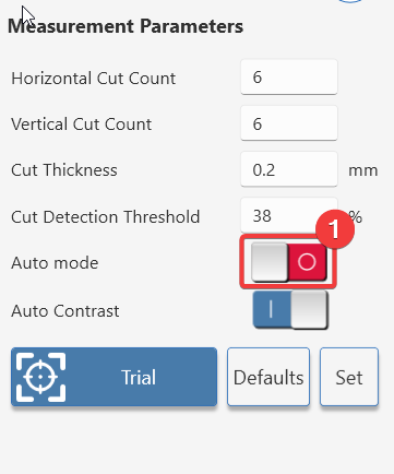
- Choose test parameters
Set grid size (1) and cut parameter (2) to match the test panel.
Move the instrument so test pattern is in the centre of the window (3).
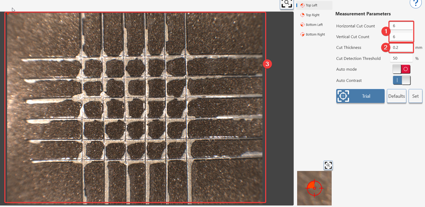
- Align the grid
- Click on the four corners of the test grid (1,2,3,4)
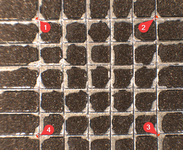
Zoom in with your mouse scroll wheel for precise placement of corners.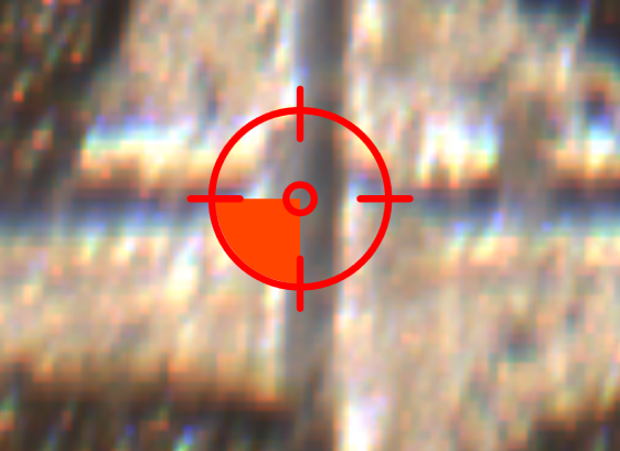
Press the set button (1) to draw the grid, check the alignment and cut thickness match the test grid (3)
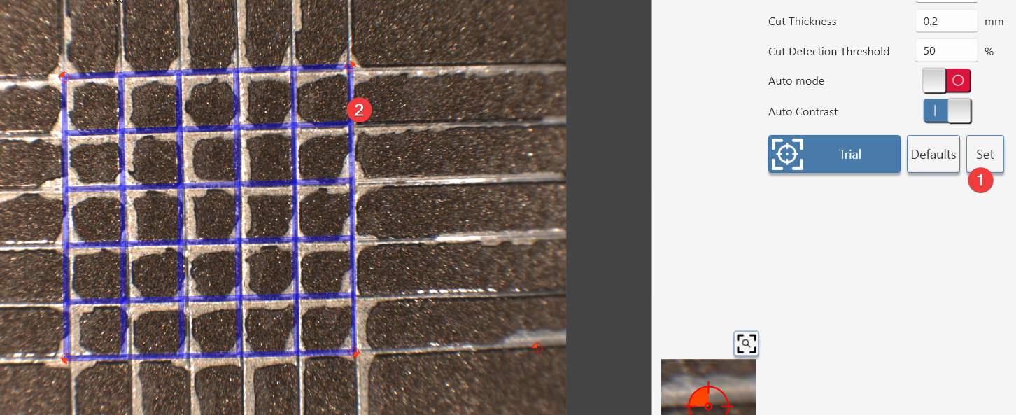
Press the trial button (1) to analyse the sample.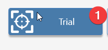
- Testing on white or light colours
The default setup detects cut lines that are lighter than the background.
When testing light colours the lines can be darker than the background.
If cut lines are darker that the background colour;
- Switch off auto contrast (1) and select invert image (2)
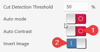
- Finetuning the detected paint area
The cut detection threshold can be adjusted to;
- Finetune a measurement so edges are more accurately defined.
- Isolate a certain colour of remaining material, for example when determining intercoat adhesion.
- Adjusting the cut detection threshold
Click on/off the found overlay (1).
The green overlay should match the area of undamaged coating.
Increasing the threshold (1) makes the detection algorithm more sensitive.
Decreasing the threshold (1) makes it less sensitive.
When the found ovelay matches the undamaged pain area;
- Click the accept measurement button (1) to include it in the table.
Cross-cut Module Measurement Guide
How Does Aesthetix Measure Cross-cut Adhesion?
The Aesthetix measures cross-cut adhesion using its Cross-cut Module, which is designed to evaluate coating adhesion strength based on the ISO 2409 standard. This involves creating a grid of cuts through the coating down to the substrate and analysing the extent of coating detachment after adhesive tape is applied and removed.
Measurement Process:
Image Capture: High-resolution images of the cross-cut area are captured
Grid Removal: The Aesthetix creates a virtual grid based on the user input on cut numbers and thiCkness, thickness, the grid is excluded from the analysis.
Analysis: The software analyses the coating detachment, identifying areas where the coating has peeled or flaked.
Quantification: Results are expressed as the percentage of remaining coating within the grid, providing an objective measure of adhesion.
This automated process ensures repeatable and accurate results, eliminating subjective errors often associated with manual evaluations.
Measurements Provided by Aesthetix for Cross-cut Adhesion
The Aesthetix provides several metrics to quantify cross-cut adhesion:
- Remaining Coating Percentage: The percentage of intact coating remaining within the cross-cut grid after testing.
- Cut Detection Threshold: Adjustable sensitivity for distinguishing adhered and detached coating areas.
- Grid Overlay Accuracy: Ensures precise alignment of the measurement grid with the cross-cut area.
Comparison and Application:
- Use Remaining Coating Percentage for general adhesion strength assessment.
- Adjust the Cut Detection Threshold for coatings with varying contrast or brightness relative to the substrate.
- For coatings with low absorption or challenging substrates, use the Invert Map setting to improve detection accuracy.
For most applications, the Remaining Coating Percentage is sufficient for quality control purposes, while threshold adjustments are useful for specific materials or substrates.
Visualising Cross-cut Adhesion Using Appearance Elements
The Rhopoint Appearance Elements software provides tools to visualise cross-cut adhesion:
- Open Cross-cut View:
- Navigate to the "Cross-cut Module" in the software.
- View a live image of the cross-cut area with an overlaid grid.
- Analyse Remaining Coating:
- Use colour-coded overlays (e.g., green for adhered areas, red for detached areas) to visualise adhesion performance.
- Adjust grid alignment or detection thresholds if needed.
- Detailed Metrics Display:
- Access quantitative results in a dedicated results panel, including remaining coating percentage and cut spacing/thickness parameters.
- Export Results:
- Save images and data for reporting or further analysis.
Improving Coating Adhesion
To improve coating adhesion:
- Surface Preparation:
- Clean surfaces thoroughly to remove contaminants like oils, dust, or residues.
- Use surface treatments such as sanding, etching, or priming to enhance mechanical bonding.
- Coating Formulation:
- Adjust binder content in paint formulations to improve adhesion properties.
- Include additives that promote better wetting and bonding with substrates.
- Application Process:
- Ensure consistent application thickness and uniformity.
- Avoid application in high humidity or extreme temperatures that could affect curing.
- Curing Conditions:
- Follow recommended curing times and temperatures to ensure proper film formation and bonding.
- Substrate Compatibility:
- Select coatings compatible with specific substrate materials (e.g., metals, plastics).
By combining these adjustments with precise measurements from Aesthetix, manufacturers can enhance coating performance and ensure compliance with quality standards.
Cross-cut Parameters
| Parameter | Description |
|---|---|
| 60° Gloss | Conventional 60° gloss value. |
| Undamaged | Percentage of the cross‑hatched test area that remains fully coated after the adhesion test; higher values indicate better coating adhesion to the substrate. |
| ASTM Class | Adhesion rating according to ASTM D3359, expressed in standard classes (for example 5B to 0B) based on the amount of coating removed in the cross-cut grid. |
| ISO Class | Adhesion rating according to ISO 2409, using ISO classes (0 to 5) to describe the degree of flaking and detachment around the cuts. |
| RGB Colour | Red, green and blue channel values from the cross-cut image, used to document the visual appearance of the test area |
Calibrating Aesthetix in AE
Once a module is chosen, it may be required to calibrate the sensor.
Calibration Standards
The following standards must be used dependent on the module.
| Module | Standard |
|---|---|
| Gloss Module | B8000-011 Gloss Module Standard |
| Texture Module | B8000-012 Texture Module Standard |
| Coatings Physical Test | B8000-011 Gloss Module Standard |
Modules which do not require calibration include:
- Sparkle Module
Click on the calibration icon to begin calibration and follow the on-screen instructions.
Calibrating an Instrument in AE
Ometrix
Taking Screen Shots
Copy and Paste
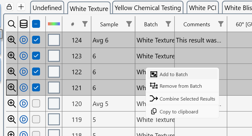
For quick and easy excel reporting, select images , right click in the table to copy and paste all the data displayed in the table.
Trouble Shooting
- Log Files
- Device Connection Problems
Log Files
This document provides information on how to locate, access, and use log files generated by the Æ Appearance Elements software.
Log files are invaluable tools for troubleshooting and problem-solving and can be retrieved from a specified directory within your system.
The following sections will guide you on how to find these files, understand their naming conventions, and employ them for effective troubleshooting.
Location
The log files for the software are located in your local drive.
You can find them in this directory: %LOCALAPPDATA%\Rhopoint Instruments Ltd\Rhopoint Appearance Elements 2\Logs.
For example, if your username is username, the full path will be:C:\Users\username\AppData\Local\Rhopoint Instruments Ltd\Rhopoint Appearance Elements 2\Logs
Accessing Log Files
To access the log files, look at the version display in the bottom right corner of the main application window.
Click on this version number to open the log files folder.
Log File Naming
The log files are named according to the date when they were generated. This allows you to easily identify logs from a specific time.
Log File Usage
Please remember that these log files can be highly helpful in troubleshooting any issues you may face. We encourage you to send them to the Rhopoint Instruments Customer Support whenever you seek help regarding any problems. The logs provide our support team with valuable information, aiding them in effectively diagnosing and addressing your concerns.
Device Connection Problems
Cable Length
When connecting devices via USB 3.0, it is recommended to use cables no longer than 3 meters to avoid common issues. Using longer USB 3.0 cables can lead to several problems due to various technical limitations. Here are the key issues:
- Signal Degradation
- Attenuation: As the length of the USB cable increases, the strength of the signal weakens due to attenuation. This can result in data transmission errors or complete failure to communicate.
- Interference: Longer cables are more susceptible to electromagnetic interference (EMI), which can further degrade the signal quality.
- Power Delivery
- Voltage Drop: Longer cables can cause a drop in voltage, leading to insufficient power being delivered to the device. This can cause devices to malfunction or not operate at all.
- Current Limitations: The resistance in the longer cables can limit the current, affecting the performance of devices that require more power.
- USB Specification Limits
- Standard Length: The USB 3.0 specification limits the maximum length of cables to 3 meters. Exceeding this length can lead to unreliable performance because the USB standard is optimized for shorter cables.
- Signal Timing: Longer cables can introduce latency in signal timing, which can disrupt the synchronous data transfer required by USB 3.0.
- Data Transfer Rates
- Reduced Speeds: The high-speed data transfer capabilities of USB 3.0 (up to 5 Gbps) can be compromised with longer cables. This can lead to reduced transfer speeds, making the connection less efficient.
- Error Rates: Increased length can raise the error rates during data transmission, leading to repeated retransmissions and thus lower effective data rates.
Solutions to mitigate USB cable problems
- Active USB Cables: These cables have built-in signal boosters or repeaters that help maintain signal integrity over longer distances.
- USB Hubs with Power: Using powered USB hubs can help maintain the necessary power levels and signal quality over extended distances by boosting the signal at each stage.
- Optical USB Cables: These convert electrical signals to light and back, reducing signal degradation and allowing for much longer cable lengths.
Using TAMS with AE
Install Appearance Elements
Connect the TAMS to AE
The Aesthetix must be connected to an available USB 3.0 port on your PC, Laptop or Windows Tablet.
TAMS Modules
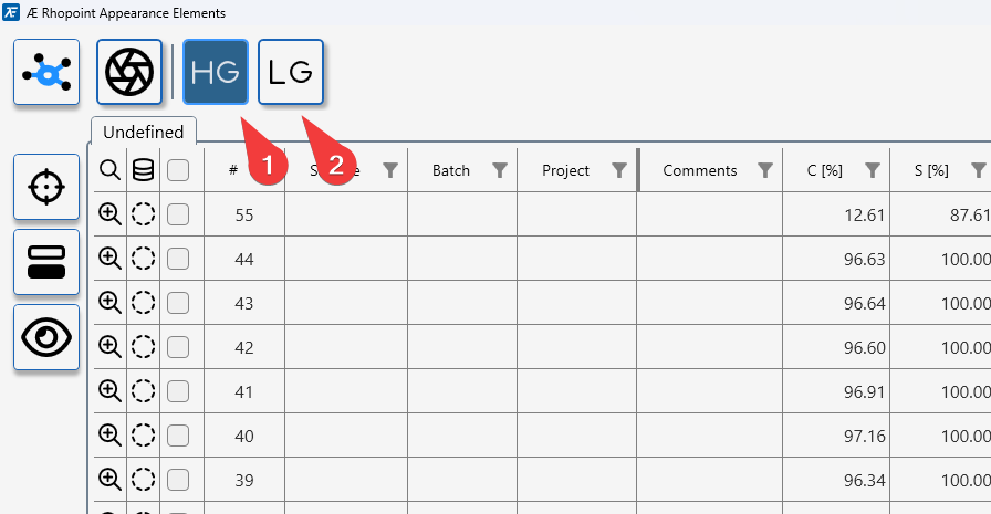
TAMS modules overview
Appearance Elements offers two TAMS modules: TAMS HG for high‑gloss, appearance‑critical surfaces and TAMS LG for low‑ to mid‑gloss, structure‑driven surfaces. Both use the same batching, statistics and reporting tools, but expose different parameters.
The available modules are determined by the licenses installed in the connected TAMS.
TAMS HG – High Gloss module
TAMS HG is used for clearcoats and other high‑gloss finishes where visual impression and matching between parts matter most. It reports Contrast, Sharpness, Waviness and Dimension, plus perception‑based Quality (Q) and Harmony (H) indices, with direct access to the underlying reflection images in the AE data table.
TAMS LG – Low Gloss module
TAMS LG is used for raw materials, E‑coat, primers and matt finishes, where surface structure and roughness dominate. It focuses on full‑field topography and waviness, providing optical roughness–style parameters from TAMS 3D maps so you can track how each process step changes the surface and relates to final appearance.
TAMS High Gloss
The TAMS HG (High Gloss) module provides a complete, perception‑based evaluation of clear‑coat and other high‑gloss surfaces by combining Contrast, Sharpness, Waviness and Dimension into the Quality (Q) and Harmony (H) indices. It is designed to show how smooth, deep and consistent a finish appears to the human eye, going far beyond simple gloss readings.
Purpose of this module
Quantify all key contributors to high‑gloss appearance, including contrast (colour impact), image sharpness, orange peel/waviness and dominant texture size on coated or polished surfaces.
Provide perception‑aligned Quality and Harmony metrics that match measured values to what people actually see, reducing disagreements between plants, suppliers and OEM appearance engineers.
Where this module can be used
High‑gloss exterior and interior coatings in automotive and commercial vehicles, including body panels, bumpers, mirrors and add‑on parts.
Other reflective products such as decorative metals, plastics, appliances and consumer goods where premium, uniform appearance across parts or assemblies is critical.
What this module measures
Contrast, Sharpness, Waviness and Dimension: Core TAMS parameters describing colour‑dependent impact, clarity of reflections, orange peel strength and dominant texture scale at showroom distance.
Quality (Q) and Harmony (H): Single‑number indices predicting overall appearance quality and the visual match between adjacent parts, so you can judge both individual surfaces and panel‑to‑panel consistency on a common scale.
How to use this module
In Appearance Elements, select the TAMS HG module, choose the appropriate job or batch, and configure TAMS for C‑Coat high‑gloss measurement using the required algorithm (for example CC‑TAMS‑STD).
Place TAMS on a clean, representative area of the surface, take one or more measurements per part, and store the results in the chosen batch; use guided or manual job modes if you want to follow a defined measurement route around a vehicle or product.
How to interpret the results
Use Quality (Q) to judge how good the high‑gloss finish appears overall and to set pass/fail limits or targets; higher Q indicates smoother, deeper, more mirror‑like surfaces.
Use Harmony (H), together with Waviness, Dimension, Contrast and Sharpness, to see whether adjacent parts match visually and to diagnose whether any mismatch is driven mainly by texture level, texture scale, colour/contrast or clarity.
TAMS High Gloss Appearance Parameters
TAMS High Gloss parameters describe how a smooth, reflective surface actually appears to a human observer, rather than just reporting traditional gloss or waviness values. Together they quantify image clarity, contrast, texture and panel‑to‑panel matching, so users can link measured numbers directly to visible differences in perceived quality.
| Parameter | Description |
|---|---|
| Quality Q | Composite quality index (0–100) that combines contrast, sharpness, waviness into a single score describing how clean, deep and mirror-like a high gloss surface appears. |
| Harmony H | Panel-to-panel matching index that quantifies how consistently different parts look to each considering differences in the amplitude of waviness and structure size. |
| Contrast C | Measures the contrast between the specular highlight and background as determined by the base paint colour. |
| Sharpness S | Describes the sharpness of reflected edges and fine detail; higher values indicate crisp, well-focused images that correlate with high DOI and premium perceived quality. High values indicate a hazy surface when viewed at 1.5m. |
| Waviness (TAMS) W | Quantifies the visual impact of orange peel viewed at 1.5m, higher values indicate more visible texture and lower perceived smoothness. |
| Dimension D | Describes the dominant wavelength of surface structure visible at a 1.5 m viewing distance, helping explain visible differences in orange peel. Low values (<2mm) indicate a surface dominated by shortwave texture, larger values (>7mm) indicate a surface dominated by longer wave texture. |
| Long-Wave Texture LW | Long-wave texture index that quantifies the visual impact of large-scale undulations and flow in the surface. |
| Short-Wave Texture SW | Short-wave texture index that describes finer-scale micro-structure on the surface; higher SW values mean more small-scale texture that can make reflections look grainy and reduce perceived smoothness. |
| DOI (TAMS) | TAMS distinctness-of-image metric that quantifies how clearly patterns are reflected on the surface; higher DOI values correspond to sharper, less distorted images and a higher perceived finish quality. |
| Gloss 20° (TAMS) | High-sensitivity 20° gloss value measured within the TAMS system, providing a conventional gloss scale for very high gloss finishes so appearance data can be linked back to existing gloss specifications. |
| Rspec (TAMS) | Peak gloss value measured in the specular highlight that is sensitive to surface texture. |
|
Elements Hub (EH)
Elements Hub
Elements Hub is a background service that makes Rhopoint instruments visible to the rest of your factory and laboratory systems. It sits between devices and third‑party software, collecting measurements and status from instruments and then sharing this information in a simple, consistent way. Typical connections include SPC and quality systems, PLCs, robots, cobots and other automation controllers that need live appearance data to make decisions.
By using Elements Hub as a single connection point, external systems do not need their own custom drivers for each Rhopoint device. Instead, they can subscribe to measurement values, pass/fail results and basic control signals from instruments such as Rhopoint Aesthetix, Rhopoint TAMS and Rhopoint ID through standard interfaces. This reduces integration effort, speeds up commissioning and makes it easier to maintain a connected appearance measurement environment over time.
The Rhopoint Elements Hub web service exposes a versioned REST API for discovering devices, controlling connected hardware, collecting measurements, and administering the hub. The API is documented via Swagger/OpenAPI and ships with an auto-configured Swagger UI at runtime. Use this guide to start the service, explore the available endpoints, and generate strongly typed clients from the OpenAPI description.
- Changelog
- Installation
- Starting the application
- Client Code Generation
- Swagger UI Guide
Changelog
The changelog for Elements Hub is publicly available online. You can view the full, up-to-date list of changes at:
https://changelog.rhopointservice.com/products/elements-hub
All change-entries are listed there, typically ordered by date or release version, so you can easily follow along from earliest releases to the most recent.
What is a Changelog
A changelog is a curated, chronologically ordered list of all the notable changes made in a project. It records enhancements, bug fixes, new features, removals, and technical adjustments. The purpose is to provide users, developers, and stakeholders with a transparent view of how the product has evolved over time.
Purpose of the Changelog
The changelog serves several key purposes:
- Transparency: Users can see what has changed, fixed, added or removed.
- Tracking Progress: Helps maintainers and contributors track what work has been completed, what remains, and what has been delivered.
- User Communication: Users can decide whether to upgrade or migrate based on what changes are relevant to them.
- Historical Reference: Provides a record for debugging, auditing, or reviewing the evolution of the product.
- Planning: Helps align future expectations by showing past patterns and the pace of development.
Installation
The latest version can be downloaded from https://download.rhopointservice.net/elements-hub
If you want to download a specific version, you can do so by specifying the version parameter, for example:
https://download.rhopointservice.net/elements-hub?version=1.6.4
Starting the application
To start the application, find it in the Start menu or locate the executable in%LOCALAPPDATA%\com.rhopointinstruments.elements-hub.release\current
Client Code Generation
This guide explains how to obtain the OpenAPI specification (swagger.json) from the Elements Hub API server and generate client code for various programming languages using OpenAPI Generator.
Getting the OpenAPI Specification
1. Access Swagger UI
The Elements Hub server provides an interactive Swagger UI interface accessible at:http://localhost:42042/swagger/
2. Download swagger.json
The OpenAPI specification is available in JSON format at:
http://localhost:42042/swagger/v1/swagger.json
You can download this file using:
curlcurl -o swagger.json http://localhost:42042/swagger/v1/swagger.json
wgetwget -O swagger.json http://localhost:42042/swagger/v1/swagger.json
PowerShellInvoke-WebRequest -Uri "http://localhost:42042/swagger/v1/swagger.json" -OutFile "swagger.json"
Client Code Generation with OpenAPI Generator
Method 1: Using Docker (Recommended)
The easiest way to generate client code is using the official OpenAPI Generator Docker image.
Basic Usage
docker run --rm \
  -v ${PWD}:/local \
  openapitools/openapi-generator-cli generate \
  -i /local/swagger.json \
  -g "generator-name" \
  -o /local/out/generated-client \
  --additional-properties=your-additional-properties
Language-Specific Examples
C# Client:
docker run --rm \
  -v ${PWD}:/local \
  openapitools/openapi-generator-cli generate \
  -i /local/swagger.json \
  -g csharp \
  -o /local/generated-client-csharp \
  --additional-properties=apiName=RhopointElementsHubClient,packageName=Rhopoint.ElementsHub.Client,nullableReferenceTypes=true,targetFramework=net9.0
C++ Client:
docker run --rm \
  -v ${PWD}:/local \
  openapitools/openapi-generator-cli generate \
  -i /local/swagger.json \
  -g cpp-restsdk \
  -o /local/out/cpp-client \
  --additional-properties=apiPackage=com.rhopointinstruments.elementshub.api,modelPackage=com.rhopointinstruments.elementshub.model,packageName=RhopointHeadlessElements
Python Client:
docker run --rm \
  -v ${PWD}:/local \
  openapitools/openapi-generator-cli generate \
  -i /local/swagger.json \
  -g python \
  -o /local/generated-client-python \
  --additional-properties=packageName=rhopoint_elements_hub_client,projectName=rhopoint-elements-hub-client
**JavaScript/TypeScript Client:**
This example uses the Angular framework.
docker run --rm \
  -v ${PWD}:/local \
  openapitools/openapi-generator-cli generate \
  -i /local/swagger.json \
  -g typescript-angular \
  -o /local/generated-client-typescript \
  --additional-properties=npmName=rhopoint-elements-hub-client
PowerShell Examples (Windows)
C# Client:
docker run --rm `
  -v ${PWD}:/local `
  openapitools/openapi-generator-cli generate `
  -i /local/swagger.json `
  -g csharp `
  -o /local/generated-client-csharp `
  --additional-properties=apiName=RhopointElementsHubClient,packageName=Rhopoint.ElementsHub.Client,nullableReferenceTypes=true,targetFramework=net9.0
Method 2: Using NPM Package
You can also install and use the OpenAPI Generator via NPM.
This example uses the Angular framework.
## Install globally
npm install -g @openapitools/openapi-generator-cli

## Generate client code
openapi-generator-cli generate \
  -i swagger.json \
  -g typescript-angular \
  -o generated-client-typescript
Supported Generators
OpenAPI Generator supports numerous programming languages and frameworks. Here are some popular options:
Client Libraries
- csharp - C# client library
- python - Python client library
- java - Java client library
- javascript - JavaScript client library
- typescript-axios - TypeScript client with Axios
- typescript-fetch - TypeScript client with Fetch API
- go - Go client library
- php - PHP client library
- ruby - Ruby client library
- swift5 - Swift 5 client library
- kotlin - Kotlin client library
- dart - Dart client library
- more
Documentation
- html2 - HTML documentation
- markdown - Markdown documentation
Automation Scripts
Bash Script for Multiple Languages
Create a script generate-clients.sh:
#!/bin/bash

## Download latest OpenAPI spec
curl -o swagger.json http://localhost:42042/swagger/v1/swagger.json

## Generate clients for multiple languages
languages=("csharp" "cpp-client" "python" "typescript-angular" "java" "go")

for lang in "${languages[@]}"; do
    echo "Generating $lang client..."
    docker run --rm \
      -v ${PWD}:/local \
      openapitools/openapi-generator-cli generate \
      -i /local/swagger.json \
      -g $lang \
      -o /local/generated-client-$lang \
      --additional-properties=packageName=RhopointElementsHubClient
done

echo "Client generation completed."
PowerShell Script for Windows
Create a script Generate-Clients.ps1:
## Download latest OpenAPI spec
Invoke-WebRequest -Uri "http://localhost:42042/swagger/v1/swagger.json" -OutFile "swagger.json"

## Define languages to generate
$languages = @("csharp", "cpp-client", "python", "typescript-angular", "java", "go")

foreach ($lang in $languages) {
    Write-Host "Generating $lang client..."
    docker run --rm `
      -v ${PWD}:/local `
      openapitools/openapi-generator-cli generate `
      -i /local/swagger.json `
      -g $lang `
      -o /local/generated-client-$lang `
      --additional-properties=packageName=RhopointElementsHubClient
}

Write-Host "Client generation completed."
Best Practices
1. Version Control
- Keep the
swagger.jsonfile in version control. - Generate clients as part of your build process.
- Tag client versions to match API versions.
- Use a wrapper project to better separate the generated client from your actual project.
2. CI/CD Integration
## Example GitHub Actions workflow
name: Generate API Clients
on:
  push:
    paths:
      - 'swagger.json'

jobs:
  generate-clients:
    runs-on: ubuntu-latest
    steps:
      - uses: actions/checkout@v3
      - name: Generate C# Client
        run: |
          docker run --rm \
            -v ${PWD}:/local \
            openapitools/openapi-generator-cli generate \
            -i /local/swagger.json \
            -g csharp \
            -o /local/clients/csharp
3. Customization
- Use custom templates when the default generation doesn't meet your needs
- Validate generated code with your coding standards
- Consider post-processing scripts for additional customization
Troubleshooting
Common Issues
Docker Volume Mounting:
- On Windows, ensure Docker Desktop has access to the drive containing your files.
- Use absolute paths if relative paths don't work.
OpenAPI Specification Validation
## Validate your OpenAPI spec
docker run --rm \
  -v ${PWD}:/local \
  openapitools/openapi-generator-cli validate \
  -i /local/swagger.json
Generator-Specific Issues:
- Check the OpenAPI Generator documentation for generator-specific options
- Use
--helpflag to see available options for each generator
Getting Help
- Review available generators: https://openapi-generator.tech/docs/generators
- Check configuration options: https://openapi-generator.tech/docs/configuration
- Community support: https://github.com/OpenAPITools/openapi-generator/issues
Swagger UI Guide
This guide explains how to use the interactive Swagger UI to explore, test, and understand the Elements Hub REST API without writing any code.
Accessing Swagger UI
1. Start Elements Hub Server
Ensure your Elements Hub server is running. By default, it runs on http://localhost:42042
2. Open Swagger UI
Navigate to the Swagger UI in your web browser: http://localhost:42042/swagger/
The server automatically redirects the root URL (/) to the Swagger UI, so you can also simply visit: http://localhost:42042

Swagger UI Interface Overview
Main Components
The Swagger UI interface consists of several key sections:
API Information Header
- API title and version
- Server information
- Base URL
Endpoint Groups (Tags)
- Organized by functionality (System, Lifecycle, Devices, etc.)
- Collapsible sections for better navigation
Individual Endpoints
- HTTP method and path
- Brief description
- Parameters and response information
Global Controls
- Authorization settings
- Server selection
- Response format options
Exploring API Endpoints
Expanding Endpoint Groups
Click on any endpoint group to expand it and see the available operations.
Understanding HTTP Methods
Each endpoint shows its HTTP method with colour coding:
- 🟢 GET (Green) - Retrieve data
- 🔵 POST (Blue) - Create or trigger operations
- 🟡 PUT (Yellow) - Update existing resources
- 🔴 DELETE (Red) - Remove resources
Viewing Endpoint Details
Click on any individual endpoint to expand its details:

Testing API Endpoints
Simple GET Request Example
Let's test the system version endpoint:
Expand the System group and click on
GET /v1/system/versionClick "Try it out" button

Click "Execute" to make the request

The response will show:
- Response Code (e.g., 200 for success)
- Response Body with the actual data
- Response Headers
- Request URL that was called

POST Request with Parameters
Let's test initialising the lifecycle services:
- Expand the Lifecycle group and click on
POST /v1/lifecycle/initialize - Click "Try it out"
- Edit the request body in the text area:
{
  "dataDirectory": "C:\\ProgramData\\ElementsHub\\Data",
  "logDirectory": "C:\\ProgramData\\ElementsHub\\Logs"
}

- Click "Execute"
POST Request with Path Parameters
For endpoints that require path parameters:
- Expand Connected Devices and click on
GET /v1/devices/{deviceId} - Click "Try it out"
- Enter the device ID in the parameter field
- Click "Execute"
Understanding Request and Response Schemas
Request Body Schemas
When an endpoint accepts a request body, Swagger UI shows:
[SCREENSHOT MARKER: Request body schema showing expandable object structure with property types and descriptions]
- Property names and their types
- Required fields (marked with *)
- Example values
- Property descriptions
You can click on the schema to see more details and copy the example JSON.
Response Schemas
Each endpoint shows possible response codes and their schemas:
- 200 Success responses with data structure
- 400 Bad Request error format
- 404 Not Found responses
- Other status codes as applicable
Working with Different Content Types
Image Responses
Some endpoints return images (like device camera captures):
Navigate to
GET /v1/devices/{deviceId}/images/latestSelect the appropriate Accept header (e.g.,
image/jpeg)Execute the request
The response will show the image data or provide a download link.
File Downloads
For endpoints that return files, Swagger UI will provide options to download or view the file content.
Error Handling and Debugging
Common Error Responses
When requests fail, Swagger UI displays helpful error information.
Request Validation Errors
If your request doesn't match the expected schema, Swagger UI will highlight:
- Missing required fields
- Invalid data types
- Out-of-range values
- Format violations
Network and Server Errors
For connectivity issues check:
- Server is running
- Correct URL and port
- Network connectivity
- Firewall settings
Advanced Features
Multiple API Versions
If multiple API versions are available, you can switch between them:
Server Selection
If multiple servers are configured, you can select which one to use:
Downloading OpenAPI Specification
You can download the raw OpenAPI specification:
Look for a link to download the swagger.json file for use with code generators.
Best Practices for Testing
1. Start with System Endpoints
Always begin by testing basic system endpoints:
GET /v1/system/version- Verify server is runningPOST /v1/lifecycle/initialize- Initialize services
2. Follow the Logical Flow
For device operations, follow this sequence:
- Initialize lifecycle services
- Start a device scan
- Check available devices
- Connect to a device
- Perform device operations
- Disconnect when done
3. Check Dependencies
Some endpoints depend on others being called first:
- Device operations require initialization.
- Device connections require scanning.
- Measurements require connected devices.
4. Use Realistic Test Data
When testing with sample data:
- Use valid file paths for directory parameters.
- Use realistic device identifiers.
- Follow the expected data formats.
5. Monitor Response Times
Pay attention to response times for operations:
- Some operations (like device scanning) may take time.
- Check for appropriate timeout handling.
- Consider async patterns for long-running operations.
Troubleshooting Common Issues
"Try it out" Button Not Working
- Ensure JavaScript is enabled in your browser.
- Check for browser console errors (press
F12on your keyboard). - Try refreshing the page.
CORS Errors
If testing from a different domain:
- CORS may need to be configured on the server or proxy.
- Try accessing from the same domain as the API.
Large Response Handling
For endpoints that return large amounts of data:
- UI may slow down or freeze.
- Responses may be truncated in the UI.
- Consider using dedicated API clients for large data sets.
- Check response size limits.
Integrating with Development Workflow
Documentation and Discovery
Use Swagger UI for:
- API Documentation - Understanding available endpoints.
- Schema Discovery - Learning request/response formats.
- Quick Testing - Validating API behaviour.
- Example Generation - Getting sample requests for development.
Code Generation Preparation
After exploring with Swagger UI:
- Download the OpenAPI specification.
- Use it with code generators (see chapter Client Code Generation).
- Reference the tested examples in your generated clients.
Tips for Effective API Exploration
1. Start Simple
Begin with read-only operations (GET requests) before attempting modifications.
2. Keep Notes
Document successful request patterns for later reference in your applications.
3. Test Edge Cases
Try invalid inputs to understand error handling and validation rules.
4. Understand State
Some operations change system state - be aware of the order of operations.
5. Use Browser Developer Tools
Monitor network requests in browser development tools for additional debugging information.
Glossary of measurement parameters
10° Sparkle Measurement
The Effect Finish module also measures how visible and intense sparkle effects appear close to the viewing direction using a 10/0 geometry, where the surface is illuminated at 10° and observed near the normal. At this near-specular angle, sparkle contributes directly to head‑on appearance, so these parameters are important for matching what users see when looking straight at an effect coating.
Density (10°)
- Density (10°): Sparkle Density 10° is the number of visible sparkle points per 100 mm² at 10°, describing how densely the surface appears filled with sparkle elements when viewed close to the observer direction.
- Higher Density (10°) values indicate a more crowded, active sparkle field in head‑on viewing.
Area (10°)
- Area (10°): Sparkle Area 10° is the average size of detected sparkle elements at 10°, representing the typical image area covered by individual sparkles in near-specular viewing.
- Larger Area (10°) values suggest coarser, more prominent sparkle particles when viewed head‑on, while smaller values correspond to a fine, pin‑point sparkle structure.
Brightness (10°)
- Brightness (10°): Sparkle Brightness 10° is the average luminance of the sparkle points at 10°, indicating how bright each sparkle appears.
- Higher Brightness (10°) values mean that individual sparkle points are more intense.
Visibility (10°)
- Visibility (10°): Sparkle Visibility 10° is the average perceived brightness of sparkle elements at 10°, taking into account their visibility and the background colour of the material.
- This parameter is designed to correlate with human perception of how noticeable the sparkle effect is in near head‑on viewing, combining contributions from density, area and brightness against the underlying coating colour.
SpR (10°), SpG (10°), SpB (10°)
- SpR (10°): Sparkle Red 10° is the red-channel intensity of sparkle elements seen at 10°, indicating how strong the red component of the sparkle appears in near head‑on viewing.
- SpG (10°): Sparkle Green 10° is the green-channel intensity of sparkle elements seen at 10°, describing the green contribution to the sparkle impression.
- SpB (10°): Sparkle Blue 10° is the blue-channel intensity of sparkle elements seen at 10°, describing the blue component of the sparkle effect in near-specular viewing.
| Parameter group | Parameter | Unit | Description |
|---|---|---|---|
| 10° sparkle metrics | SpR (10°) | Intensity (0–255) | Red‑channel sparkle intensity at 10°, indicating how strong the red component of the sparkle appears in near head‑on viewing. |
| SpG (10°) | Intensity (0–255) | Green‑channel sparkle intensity at 10°, describing the green contribution to the sparkle impression. | |
| SpB (10°) | Intensity (0–255) | Blue‑channel sparkle intensity at 10°, describing the blue component of the sparkle effect in near-specular viewing. | |
| Density (10°) | 1/100 mm² | Number of visible sparkle points per 100 mm² at 10°, describing how densely the surface appears filled with sparkle elements. | |
| Area (10°) | mm² | Average size of detected sparkle elements at 10°, representing the typical image area covered by individual sparkles. | |
| Brightness (10°) | AU* | Average luminance of the sparkle points at 10°, indicating how bright each sparkle appears relative to the surrounding surface. | |
| Visibility (10°) | AU* | Average perceived brightness of sparkle elements at 10°, taking into account their visibility and the background colour of the material. |
*AU = arbitrary (instrument) units.
60° Gloss (Aesthetix)
Parameter description
Definition: Gloss refers to the overall shiny appearance of a surface when light is reflected directly off it. It is often measured using glossmeters which quantify the amount of reflected light at specific angles.
Importance: Gloss is the most widely used measure of a surface's ability to reflect light in a specular manner, contributing to its shiny appearance.
High gloss values indicate bright, mirror-like finishes, while low values indicate matt or dull surfaces.
How is it measured?
Aesthetix specular light source (1) projects a controlled light beam onto the surface (2) at 60° and captures the reflected intensity with the gloss camera (3).
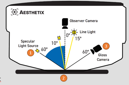
The optical layout of the gloss sensor
The signal is compared to a calibrated reference standard and expressed in gloss units, measurements comply to ISO2813 & ASTM D523, the recognised standards for gloss measurement.
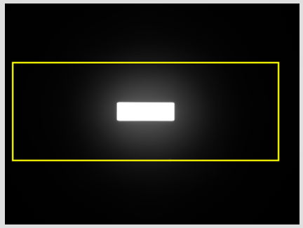
**Specular reflection from a calibration standard captured by the gloss camera. To comply with the angular tolerances in the standard, light in the yellow area is integrated. **
Applications
Routine control of high-gloss, semi-gloss and matt coatings in automotive, furniture, plastics, packaging and consumer goods.
Verifying that production parts match master panels or customer specifications for gloss level before shipment.
Technical specifications
| Item | Specification / Value |
|---|---|
| Gloss index | 60° Gloss (all Aesthetix modules that report gloss) |
| Gloss unit | GU (Gloss Units) |
| Measurement geometry | 60° specular gloss geometry |
| Field of view (FOV) | 18 × 24 mm |
| Standard analysed gloss area | 18 × 9 mm |
| Optional small gloss spot | 4 × 2 mm |
| Other analysed areas (modules) | Effect Finish: 10 × 10 mm; Texture: up to 15 × 15 mm; Polishing Quality: 10 × 10 mm |
| Surface resolution | 9.2 µm/pixel (109 pixels/mm) |
| Repeatability, 0–10 GU | ±0.1 GU |
| Repeatability, 10–100 GU | ±0.2 GU |
| Repeatability, 100–1000 GU | ±0.2% of reading |
| Reproducibility, 0–10 GU | ±0.2 GU |
| Reproducibility, 10–100 GU | ±0.5 GU |
| Reproducibility, 100–1000 GU | ±0.5% of reading |
These repeatability and reproducibility values assume correct calibration on a certified gloss tile, stable environmental conditions and consistent sample positioning and measurement practice.
45° Sparkle Measurement
The Effect Finish module quantifies how visible and intense sparkle effects appear when an effect coating is viewed at a 45/0 geometry, i.e. illuminated at 45° and observed close to the normal. At this angle, sparkle is often more pronounced and directional, so these parameters are particularly useful for matching appearance in real-world viewing conditions on automotive and other effect-coated parts.
SpR (45°), SpG (45°), SpB (45°)
- SpR (45°): Sparkle Red 45° is the red-channel intensity of sparkle elements seen at 45°, indicating how strong the red component of the sparkle appears at this off‑specular angle.
- SpG (45°): Sparkle Green 45° is the green-channel intensity of sparkle elements seen at 45°, describing the green contribution to the sparkle impression.
- SpB (45°): Sparkle Blue 45° is the blue-channel intensity of sparkle elements seen at 45°, describing the blue component of the sparkle effect.
Density (45°)
- Density (45°): Sparkle Density 45° is the number of visible sparkle points per 100 mm² at 45°, describing how densely the surface appears filled with sparkle elements when viewed from this angle.
- Higher Density (45°) values indicate a busier, more active sparkle field, whereas lower values correspond to a sparser, more subtle effect.
Area (45°)
- Area (45°): Sparkle Area 45° is the average size of detected sparkle elements at 45°, representing the typical image area covered by individual sparkles.
- Larger Area (45°) values suggest coarser, more prominent sparkle particles, while smaller values correspond to fine, pin‑point sparkle.
Brightness (45°)
- Brightness (45°): Sparkle Brightness 45° is the average luminance of the sparkle points at 45°.
- Higher Brightness (45°) values mean that individual sparkle points are more intense.
Visibility (45°)
- Visibility (45°): Sparkle Visibility 45° is the average perceived brightness of sparkle elements at 45°, taking into account their visibility and the background colour of the material.
- This parameter is designed to correlate with human perception of how noticeable the sparkle effect is at 45°, combining contributions from density, area and brightness against the underlying coating colour.
| Parameter group | Parameter | Unit | Description |
|---|---|---|---|
| 45° sparkle metrics | SpR (45°) | Intensity (0–255) | Red‑channel sparkle intensity at 45°, indicating how strong the red component of the sparkle appears at this off‑specular angle. [3] |
| SpG (45°) | Intensity (0–255) | Green‑channel sparkle intensity at 45°, describing the green contribution to the sparkle impression. [3] | |
| SpB (45°) | Intensity (0–255) | Blue‑channel sparkle intensity at 45°, describing the blue component of the sparkle effect. [3] | |
| Density (45°) | 1/100 mm² | Number of visible sparkle points per 100 mm² at 45°, describing how densely the surface appears filled with sparkle elements. [3] | |
| Area (45°) | mm² | Average size of detected sparkle elements at 45°, representing the typical image area covered by individual sparkles. [3] | |
| Brightness (45°) | AU* | Average luminance of the sparkle points at 45°, indicating how bright each sparkle appears relative to the surrounding surface. [3] | |
| Visibility (45°) | AU* | Average perceived brightness of sparkle elements at 45°, taking into account their visibility and the background colour of the material. [3] |
*AU = arbitrary (instrument) units.
Ca- Cell Amplitude
Ca (reported in [p-µm] (perceived microns)) is defined as the average amplitude of all cells features identified within the texture of a material.
It quantifies the difference between the highest and lowest points, (Average Height of cells- Average Depth of valleys) providing a measure of the vertical dimension of the texture.
This parameter is used to understand the depth and relief of the surface texture, which directly influences visual and tactile perception.
A higher cell amplitude indicates a more pronounced texture, lower values will be measured on smoother materials.
Unit- Perceived Microns [pµm]
Cn- Cell Number
Cn refers to the total number of distinct cells or surface features identified within the field of measurement depending on the watershed parameters set.
This measurement is crucial for understanding the density and distribution of the texture features, which influence visual and tactile qualities.
Cs—Mean Cell Size
Mean Cell Size is the average size of the cells included in the analysis, measured in square millimeters [mm²].
To find this value, the areas of all included cells are measured, and their mean (average) value is calculated. It provides an overall sense of the typical size of the structural features on the surface.
CsDev—Cell Size Standard Deviation
The Cell Size Standard Deviation reflects the variation in cell sizes across the surface.
By dividing the standard deviation by the mean cell size, the resulting value is normalized, allowing for comparability between different types of structures.
This index indicates how much the sizes of the cells vary from the average, helping to understand the consistency of the surface structure.
CsMax—Maximum Cell Size
CsMin—Minimum Cell Size
Cell Size Minimum represents the size of the smallest cell among all those included in the data analysis.
It gives insight into the minimum limit of the structural features present on the surface.
DOI Distinctness of Image (Aesthetix)
DOI (Distinctness of Image) is a surface appearance parameter that describes how clearly objects and edges are reflected in a glossy surface.
Parameter description
DOI indicates the sharpness of reflected images: high DOI means crisp, mirror‑like reflections, while low DOI indicates blurred, distorted or surfaces where orange‑peel distorts reflections. It is expressed as a percentage, with 100% representing an ideal mirror and lower values representing increasing loss of image clarity.
How is it measured?
Software analyses the reflected gloss image, a sharp, well‑defined image yields high DOI, a blurred gloss image will return lower values.
Applications
Assessing and optimising the visual quality of automotive bodywork, bumpers and high‑gloss trim where mirror‑like reflections are critical.
Controlling polishing, sanding and coating processes for premium furniture, pianos, consumer electronics and decorative plastics to minimise orange peel and achieve a high‑quality finish.
DOI is a crucial value for polished stone and concrete applications.
DOI values are correlated between Rhopoint Aesthetix and Rhopoint IQ measurement systems.
| Item | Specification / Value |
|---|---|
| Index name | DOI |
| Description | Measures how clearly and sharply images and edges are reflected from a surface |
| Unit | % (0–100%, where 100% represents a perfectly sharp, undistorted reflection) |
| Measurement geometry | Specular reflection geometry (typically 60° or 20°, depending on module/instrument) |
| Measurement principle | Analysis of the spread and distortion of reflected light around the specular angle |
| Field of view (FOV) | 18 × 24 mm (Aesthetix optical head) |
| Standard analysed area | 18 × 9 mm (shared with gloss/DOI measurements) |
| Optional small spot | 4 × 2 mm (small‑area adapter, where available) |
| Other analysed areas | Effect/texture modules up to 10 × 10 mm or 15 × 15 mm, depending on configuration |
| Measurement range | 0–100% |
| Repeatability (typical) | ±0.2% DOI |
| Reproducibility (typical) | ±0.5% DOI |
| Primary use | Quantifying orange peel, surface smoothness and image clarity on high‑gloss finishes |
F—Fill Factor
The Fill Factor index represents the ratio of the mean hill size to the mean cell size, expressed as a percentage.
It provides a measure of how much of the cell area is occupied by hills, indicating the density of the elevated structures on the surface or distance between structures.
Graininess
Graininess describes how coarse or fine an effect coating appears under diffuse viewing conditions, similar to looking at a panel outside on a cloudy day when the light is spread evenly across the sky. In this situation and the underlying flake texture of the coating becomes more visible than sharp, directional sparkle from the metallic particles.
What Graininess represents
- Graininess quantifies the low‑frequency mottling or speckle pattern caused by non-uniform flake distribution and local brightness variations across the surface that are most apparent under diffuse conditions.
- Higher Graininess values indicate a more visibly textured, patchy or “noisy” effect, while lower values indicate a more uniform, fine and homogeneous finish.
How Graininess is measured
- The parameter is derived from the spatial variation in reflected intensity within the measured area, using data from all six illumination directions and processing it to remove specular contributions from the sparkling elements.
How to use Graininess in practice
- Use Graininess, referenced to diffuse viewing conditions (cloudy‑day type lighting), to set and check appearance specifications for metallic and pearlescent coatings, ensuring that production parts match master panels in perceived coarseness under typical daylight, showroom or indoor lighting.
- Compare Graininess alongside sparkle metrics and waviness to separate diffuse‑appearance texture issues (e.g. layout, flocculation) from directional sparkle behaviour when diagnosing or optimising effect coatings.
Technical specification
| Parameter | Description |
|---|---|
| Graininess | Quantifies how coarse or fine an effect coating appears under diffuse, cloudy‑day type viewing conditions. |
| Viewing mode | Assessed under diffuse illumination so that sparkle is suppressed and the underlying flake texture becomes more visible. |
| Measurement principle | Derived from the spatial variation in reflected intensity within the measured area, using data from all six illumination directions and processing it to remove specular contributions from sparkling elements. |
| Visual meaning | Higher values indicate a more mottled, noisy or patchy look; lower values indicate a smoother, more uniform and silky appearance. |
| Typical use | Used to set and check appearance specifications for metallic and pearlescent coatings to simulate viewing in diffuse, cloudy‑day conditions. |
Haze and Compensated Haze
Parameter description
Haze describes the scattering of light by a surface that creates a milky halo around the main reflection and reduces contrast in the reflected image. It diminishes the perceived depth and clarity of high‑gloss finishes and is usually undesirable on premium surfaces.
Haze (C), often reported as LogH C, is a compensated haze parameter that corrects for the influence of background colour and diffuse reflection, providing a more stable haze value across different colours and effects.
How is it measured?
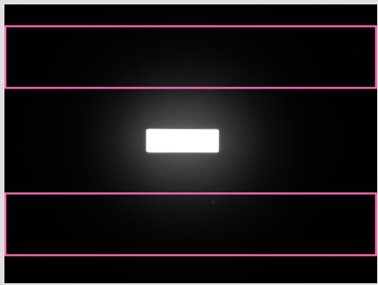
**
Haze is calculated by measuring the amount of light in the near specular region (pink area) and comparing it to calibration values. Log Haze (C) combines this with luminosity values from the observer camera**
The Aesthetix sensor captures a high‑dynamic‑range image of the specular reflection at 60° and analyses the distribution of light around the main gloss peak.
Haze is quantified from the amount of light present in defined off‑specular regions (typically a few degrees either side of the specular angle), generating a base haze value.
Haze (C) / LogH C is then calculated by applying a logarithmic and colour‑compensated transformation to the haze data, reducing the impact of underlying shade and diffuse reflection and aligning the scale with familiar Rhopoint gloss‑haze conventions.
Applications
Quality control of high‑gloss and dark coatings in automotive, electronics and decorative applications, where even low levels of haze are visually obvious.
Monitoring polishing, clearcoat formulation and process conditions to minimise cloudiness and maintain a deep, clear “wet look” finish on premium products and furniture.
Routine production monitoring and specification setting where parts of different colours, tints or metallic content must be compared using a single, robust haze scale, especially for Class A surfaces such as body panels, appliances and high‑end furniture.
Technical Specifications
| Item | LogH (Log Haze) | LogH C (Log Haze compensated) |
|---|---|---|
| Index name | LogH | LogH C |
| Description | Logarithmic reflection haze | Logarithmic reflection haze with colour compensation |
| Unit | logHU | logHU |
| Measurement geometry | 60° specular, off‑specular bands near gloss angle | 60° specular, off‑specular bands near gloss angle |
| Field of view (FOV) | 18 × 24 mm | 18 × 24 mm |
| Standard analysed area | 18 × 9 mm | 18 × 9 mm |
| Optional small spot | 4 × 2 mm | 4 × 2 mm |
| Measurement range (typical) | 0–500 logHU | 0–500 logHU |
| Repeatability (typical) | ±1 logHU | ±1 logHU |
| Reproducibility (typical) | ±10 logHU | ±10 logHU |
| Primary use | Historical specifications only | Routine QA and specifications where colour‑independent haze values are needed |
Hs—Hill Size
This is the average cross-sectional area of the hills within the analyzed cells, measured in square millimetres [mm²].
The algorithm detects the cross-sections of the hills and calculates the mean area. The threshold height used to define the cross-sections is parameterized, meaning it can be adjusted based on specific analysis requirements.
Understanding hill size helps in evaluating the distribution and prominence of these elevated features.
Michelson Contrast Haze MCH
MCH (Michelson Contrast Haze) is a visual haze parameter that quantifies the loss of contrast between the specular highlight and its surrounding area using the Michelson contrast formula, closely matching how hazy the surface appears to the eye.
Parameter description
MCH describes how much the halo around the specular highlight reduces the contrast between bright and dark regions in the reflected image. A low MCH value indicates a sharp, well‑defined highlight with high contrast, while a higher MCH value indicates a hazier surface with a broader, more washed‑out highlight.
How is it measured?
The instrument captures a high‑dynamic‑range image of the gloss highlight and the neighbouring background at the 60° geometry.
Michelson contrast is calculated from the luminance of the bright highlight region and the adjacent darker region, and this contrast value is converted into the MCH haze scale used for reporting and comparison.
Applications
Characterising visual haze on high‑gloss coatings where small differences in haze and contrast are seen by observers but not well captured by traditional haze scales.
Setting appearance limits and monitoring production for premium automotive, electronics and decorative finishes, ensuring that perceived haze remains within acceptable visual tolerances.
| Item | Specification / Value |
|---|---|
| Index name | MC H (Michelson Contrast Haze) |
| Metric type | Visual haze based on Michelson contrast of the specular highlight and adjacent regions |
| Unit | HU (Haze Units) |
| Measurement geometry | 60° specular, contrast evaluated between highlight and near specular haze region |
| Standard analysed area | 18 × 9 mm |
| Optional small spot | 4 × 2 mm |
| Measurement range | 0–150 HU (typical working range) |
| Repeatability (typical) | ± 0.2HU |
| Reproducibility (typical) | ± 0.5 HU |
| Primary use | Quantifying visually perceived haze/halo around highlights on high‑gloss surfaces |
R—Reflectivity
The Mean Reflectivity index R represents the average reflectivity value of the surface, or a value for how the surface interacts with light, contributing to its visual characteristics such as gloss and brightness.
Reflectivity is an absolute measurement but uses a non-standard unit (arbitrary units [arb'U]) specific to the measurement system.
RC—Reflective Contrast
This index quantifies the difference in reflectivity between the hills and valleys of the surface topography.
The algorithm separates the surface data into valleys and hills using a parameterized threshold height.
It then calculates the mean reflectivity values for both areas and uses the contrast formula:
contrast = (hill + valley) / (hill − valley)
This provides a measure of how much the reflectivity differs between the elevated and depressed areas of the surface.
RH—Reflectivity on Hills
This is the average reflectivity value specifically for the areas classified as hills.
It provides insight into the reflectivity characteristics of the elevated parts of the surface.
RGB Colour
RGB Colour records the basic colour information of the surface image as three separate channels: red (R), green (G) and blue (B).
Parameter description
RGB Colour describes the appearance of the surface in terms of its digital image colour values rather than in a colour‑space such as CIELab. Each pixel in the observer‑camera image has an R‑G‑B triplet; the reported RGB Colour values are the average red, green and blue channel intensities over the analysed area, giving a simple numerical description of surface shade and tone.
How is it measured?
- The observer camera captures a colour‑corrected image of the surface using 45° circumferential illumination and 0° observation geometry.
- Software averages the red, green and blue pixel values within the defined measurement area (for example 18 × 9 mm), reporting three numbers: R, G and B. These values can be trended, compared between batches or exported for further colour analysis.
Interpretation of values
- Higher R values indicate a stronger red component, higher G values a stronger green component, and higher B values a stronger blue component in the surface colour.
- Changes in RGB channel balance over time or between samples indicate colour drift, contamination, ageing or process variation, even when gloss and texture remain constant.
Applications
- Monitoring batch‑to‑batch colour consistency of coatings, plastics, inks and decorative films alongside gloss, haze and texture metrics.
- Quickly flagging visible colour shifts on production lines or during development trials without needing a dedicated spectrophotometer, and documenting the appearance of standards, master panels and reference parts in quality systems.
Technical Specification
| Item | Specification / Value |
|---|---|
| Index names | R, G, B |
| Description | Average red, green and blue channel intensities from the surface image |
| Units | 0–255 (8‑bit channel values) or normalised 0.0–1.0, depending on software configuration |
| Measurement geometry | 45° circumferential illumination, 0° observation (observer camera) |
| Field of view (FOV) | Dependent on module |
| Measurement principle | Capture of a colour image, followed by spatial averaging of R, G and B pixel values over the region |
| Measurement range | Full sensor range for each channel (typically 0–255) |
| Repeatability (typical) | Within ±1–2 channel |
| Reproducibility (typical) | Within ±3–5 channel counts after re‑positioning and re‑measurement |
| Primary use | Tracking colour/shade changes and documenting appearance alongside gloss, haze and texture parameters |
RV—Reflectivity in Valleys
This index represents the average reflectivity value for the areas classified as valleys. The centre of the valleys are represented by red lines on the feature maps.
It helps in understanding the reflectivity properties of the lower, depressed regions of the surface.
Sa Rough – Areal Surface Roughness
Sa Rough – Areal Surface Roughness describes the average height variation of the surface over the full measured area, expressed in perceived microns (p‑µm) to reflect how roughness is seen in the Aesthetix texture image.
The calculation uses unfiltered topographical information from the full 3D height map, so all peaks and valleys in the measurement area contribute to the result rather than a smoothed or wavelength‑limited profile.
Lower Sa values indicate a smoother, more level surface, while higher values correspond to a rougher finish with more pronounced structure or texture.
Unit- Perceived Microns [pµm]
Scratch Parameters
How scratches are detected
- Scratches are detected using a high‑intensity 10° spot light that illuminates the surface in a very directional way, similar to shining an inspection torch across a panel to reveal fine marks.
- An observer camera captures a high‑resolution image of the illuminated area, and image‑processing algorithms analyse the bright, elongated features caused by light catching on scratch edges.
Role of sensitivity
- The Sensitivity setting controls how aggressively the system looks for scratches by adjusting detection thresholds in the image analysis.
- At low sensitivity, only the more obvious scratches are reported, corresponding to defects that are easily visible under typical indoor or workshop lighting.
- At medium sensitivity, the system reveals finer swirls and lighter polishing marks that may be visible under stronger point light sources, for example inspection lamps or showroom lighting.
- At the highest sensitivity, the algorithm highlights almost all detectable line structures, including very faint scratches and holograms that may only become visible under high illuminance conditions, such as bright sunshine or intense inspection lighting.
Length, Length V and Length H
- Length – Scratch Length Total Average (µm): The average total length of all detected scratches within the measured area, giving an overall indication of how extensive linear defects are on the surface.
- Length V – Scratch Length Average Vertical (µm): The average total length of scratches predominantly aligned in the vertical direction, useful for identifying directionality from specific polishing passes or tools.
- Length H – Scratch Length Average Horizontal (µm): The average total length of scratches predominantly aligned in the horizontal direction, highlighting directional polishing patterns.
Area, Area V and Area H
- Area – Total Scratched Area (µm²): The combined surface area covered by all detected scratches, indicating how much of the inspected region is affected by polishing defects.
- Area V – Scratched Area Vertical (µm²): The total area occupied by vertically oriented scratches, helping to separate their contribution from other defect directions.
- Area H – Scratched Area Horizontal (µm²): The total area occupied by horizontally oriented scratches, useful when diagnosing process steps that introduce specific directional marks.
Count, Count V and Count H
- Count – Total Scratches (–): The number of individual scratches detected in the measurement, giving a simple measure of how densely the surface is covered with defects.
- Count V – Scratches Vertical (–): The number of vertically oriented scratches, used to identify and track polishing steps that introduce mainly vertical marks.
- Count H – Scratches Horizontal (–): The number of horizontally oriented scratches, indicating the prevalence of defects aligned with horizontal polishing movements.
Visibility, Visibility V and Visibility H
- Visibility – Scratch Visibility Average (AU): The average perceived visibility of all detected scratches, combining their brightness, contrast and size into a single perception‑based value.
- Visibility V – Scratch Visibility Vertical (AU): The perceived visibility of vertically oriented scratches, highlighting whether vertical marks are particularly noticeable to the observer.
- Visibility H – Scratch Visibility Horizontal (AU): The perceived visibility of horizontally oriented scratches, allowing judgement of whether horizontal swirls or holograms dominate the visual impression.
Sharpness (Aesthetix)
Sharpness is a surface appearance parameter that quantifies how clearly and crisply a surface reflects fine detail and edges in a mirrored image.
Parameter description
Sharpness indicates the edge clarity within a reflection rather than the overall brightness or gloss level. High sharpness values correspond to very clear, well‑defined edges and fine details in the reflected image, while low values indicate blurred, smeared or “soft” reflections that reduce the perceived quality and depth of finish.
How is it measured?
- The instrument illuminates the surface and captures a high‑resolution image of a reflected pattern or highlight at the specular geometry.
- Software analyses edge transitions and local contrast within the reflected pattern; sharp, high‑contrast edges produce high sharpness values, whereas widened, low‑contrast edges reduce the sharpness value, which is typically reported on a 0–100 scale.
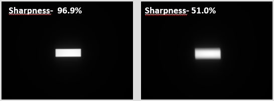
Sharpness measures the clarity of sharp edges visible in a reflection and is exceptionally sensitive to ultra-fine structures that only become visible at close viewing distances (typically under 20cm). In the example, two high-gloss surfaces show similar gloss and DOI values but the surface on the right has subtle micro-texture that softens edges in the reflection, reducing the quality of the finish.
Difference between Sharpness and DOI
- Sharpness concentrates on the local edge definition in the reflection, making it very sensitive to small amounts of blurring that soften fine details and lines.
- DOI (Distinctness of Image) evaluates the overall fidelity of the reflected image, responding more strongly to broader spreading and distortion caused by orange peel and larger‑scale texture than to subtle edge softening.
Applications
- Evaluating polishing quality and surface finish on automotive bodywork, piano and furniture lacquers, consumer electronics and decorative plastics where mirror‑like clarity is critical.
- Monitoring process changes (substrate preparation, coating formulation, application and curing) to minimise micro‑texture and orange peel that reduce edge clarity, ensuring consistent premium appearance across parts and batches.
Technical Specification
| Item | Specification / Value |
|---|---|
| Index name | S (Sharpness) |
| Description | Measures the clarity and definition of sharp edges and fine details visible in the reflected image |
| Unit | % (0–100%, higher values = crisper reflections) |
| Measurement geometry | Specular reflection at 60° (shared with gloss/DOI) |
| Measurement principle | Image‑based analysis of local edge contrast and edge width in the reflected pattern |
| Standard analysed area | 18 × 9 mm |
| Optional small spot | 4 × 2 mm |
| Other analysed areas | Effect / Texture / Polishing modules: up to 10 × 10 mm or 15 × 15 mm, depending on configuration |
| Sensitivity | Highly sensitive to ultra‑fine surface texture visible at viewing distances below ~20 cm |
| Measurement range | 0–100% |
| Repeatability (typical) | ±0.2% sharpness |
| Reproducibility (typical) | ±0.5% sharpness |
| Primary use | Discriminating very high‑gloss finishes by edge clarity, revealing micro‑texture not seen in gloss alone |
Visual Gloss
Parameter description
Visual Gloss is a perception-based gloss value that predicts how glossy a surface appears to the human eye, rather than just how much light it reflects in a single direction. It adjusts for effects such as colour, highlight contrast and surrounding brightness so that the scale better matches visual judgements across different materials and finishes.
How is it measured?
The Aesthetix sensor captures a high dynamic range (HDR) image of the specular highlight and surrounding area at the standard 60° gloss geometry. The observer camera captures an image of the surface and measures its luminosity.
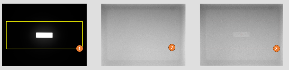
Reflection data from the gloss camera (1) is virtually combined with surface luminosity information from the observer camera (2) the result is visual gloss which describes the contrast of the gloss highlight against the background colour (3).
Software analyses intensity of the highlight and the background into a Visual Gloss value on a perceptual scale.
Applications
Comparing gloss across different colours, coatings and substrates where standard gloss units do not reliably match what observers see.
Setting appearance specifications and pass/fail limits for premium high‑gloss products (automotive, electronics, furniture, decorative parts) using a metric that closely tracks customer perception.
Technical Specifications
| Item | Specification / Value |
|---|---|
| Visual gloss index | 60° Visual Gloss (60° V) |
| Visual gloss unit | p‑GU (perceptual gloss units) |
| Measurement geometry | 60° specular geometry with HDR image capture |
| Field of view (FOV) | 18 × 24 mm |
| Standard analysed visual‑gloss area | 18 × 9 mm |
| Optional small visual‑gloss spot | 4 × 2 mm |
| Repeatability, typical | Equivalent to ±0.2 GU over the 10–100 GU gloss range (expressed on the p‑GU scale) |
| Reproducibility, typical | Equivalent to ±0.5 GU over the 10–100 GU gloss range (expressed on the p‑GU scale) |
Visual Haze
Visual Haze Indoors and Outdoors are perception-based haze values that describe how hazy a high‑gloss surface appears under typical indoor or outdoor lighting conditions.
Parameter description
Visual Haze values indicate the loss of contrast and clarity around the specular highlight, expressed on a dedicated VHU scale. Visual Haze Indoors is tuned for viewing under common interior lighting (artificial light, lower illuminance), while Visual Haze Outdoors is tuned for brighter, directional daylight where halos and cloudiness are more noticeable.
How are they measured?
The instrument captures a high‑dynamic‑range image of the specular reflection and adjacent regions at the 60° geometry.
Software processes the image using different luminance and contrast weightings that represent indoor or outdoor viewing conditions, converting the result into Visual Haze Indoors (VHU) and Visual Haze Outdoors (VHU) values.
Applications
Visual Haze Indoors: specification and quality control of products primarily viewed under indoor lighting, such as interior automotive trim, furniture, domestic appliances and electronic devices.
Visual Haze Outdoors: evaluation of exterior body panels, coated metalwork, signage and other surfaces exposed to daylight, ensuring that haze remains within acceptable limits in bright outdoor conditions.
Unit: Perceived Microns [pµm]
The unit "perceived" is calculated from Photometric Stereo Topographical maps from the surface slopes and facets that are visible to the camera and calibrated using a 540µm artifact.
Our optical system works best for surfaces with a texture amplitude of 0-1500 (1.5mm) microns with homogeneous reflectivity- in this range the Aesthetix measurement system is linear and obtains results highly correlated to other systems.
Waviness (Aesthetix)
Waviness is a surface appearance parameter that quantifies the strength of orange peel – surface waves that distort reflections on otherwise glossy surfaces.
Parameter description
Waviness describes larger‑scale texture features on the surface (typically in the 0.1–10 mm range) that cause reflected straight lines to appear wavy rather than perfectly straight. Higher waviness values indicate more pronounced orange peel and a more obviously distorted reflection, while lower values correspond to smooth, piano‑like finishes with minimal visible structure.
How is it measured?
- The instrument projects a line or pattern onto the surface and records the reflected image using the observer camera.
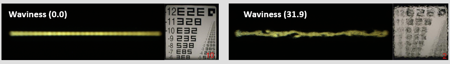
The distortion of the reflected of a straight line is captured by the observer camera. The visual effect of orange peel can seen in the reflected test charts on the right of the camera images.
- Software analyses how much the reflected line deviates from a mathematically straight reference; these deviations are converted into a waviness value (WU) that is calibrated to align with perception‑based orange‑peel scales at a typical viewing distance of around 1.5 m.
Interpretation of values
- Very low WU values correspond to “piano finish” surfaces with virtually no visible orange peel and a strong impression of quality.
- Increasing WU values move through low, standard and high orange‑peel ranges, where the texture becomes clearly visible and increasingly negative for perceived surface quality, especially on dark, high‑gloss colours.
Applications
- Setting and monitoring orange‑peel targets on automotive body panels, bumpers, commercial vehicles and yacht coatings to match appearance standards.
- To improve wavines- optimise coating systems, spray parameters, viscosity and curing conditions, waviness may also "telegraph" through from an imperfect substrate.
Here is a parameter table for Waviness:
| Item | Specification / Value |
|---|---|
| Index name | Waviness |
| Unit | WU (Waviness Units) |
| Description | Quantifies orange peel –surface undulations that distort reflections |
| Measurement geometry | Specular reflection using projected line light and observer camera at fixed distance and angle |
| Analysed distance | 20mm line on surface. mm |
| Other analysed areas | Effect / Texture / Polishing modules: up to 10 × 10 mm or 15 × 15 mm, depending on configuration |
| Perceptual basis | Scale aligned to human perception of orange peel at ~1.5 m viewing distance (correlated to Rhopoint TAMS scale) |
| Typical value ranges (automotive) | < 2 WU: piano finish; 2–5 WU: low orange peel; 5–10 WU: standard orange peel; 10–15 WU: high orange peel |
| Measurement range | Approx. 0–30 WU |
| Repeatability (typical) | ±0.5 WU |
| Reproducibility (typical) | ±1.0 WU |
| Primary use | Setting and monitoring orange‑peel levels on high‑gloss coatings such as automotive, marine and furniture |
Quality (TAMS High Gloss)
Quality (Q) – High gloss mode
Definition
Quality (Q) is a perception-based index that describes the overall visual appearance of a high gloss clear-coat surface. It combines contrast, sharpness and waviness into a single value that reflects how good or bad the finish looks to an observer.
Unit and range
Q is expressed in percent (%), from 0% (very poor, strongly distorted reflections) to 100% (mirror-like, premium appearance). Typical automotive clear-coats fall between these extremes depending on process and substrate.
Measurement conditions
Q is available in High Gloss Mode when the surface type is set to C-Coat and the CC‑TAMS‑STD algorithm is selected on TAMS. Measurements should be taken on near-flat, clean, defect-free areas; at least three readings are recommended before closing the batch to obtain averaged Q results.
Related parameters
The following sub-parameters are calculated for each measurement and used to derive Q:
- Contrast (C): Relative intensity difference between bright and dark areas in the reflected pattern, 0–100%. Higher values indicate deeper, more vivid reflections.
- Sharpness (S): Clarity of the reflected image across viewing distances, 0–100%. Lower values indicate haze or blurred reflections.
- Sharpness-Q (Sq): Internally scaled sharpness term (0–100%) used by the Quality algorithm; not normally displayed.
- Waviness (W): Degree of large-scale surface undulation or orange peel, typically from 0 (flat) to around 30 (very wavy).
- Dimension (D): Dominant structure size perceived at typical viewing distance, reported in millimetres.
Computation principle
Q is calculated using a proprietary algorithm that combines Contrast, Sharpness (including Sq) and Waviness to match human visual grading of clear-coat appearance. Higher contrast and sharpness increase Q, while higher waviness reduces it.
Colour dependence and advantage
An important advantage of the TAMS Quality index is that the basecoat colour is inherently taken into account through the contrast term when calculating Q. This allows Quality to be assessed consistently across different colours instead of assuming that all colours behave like a neutral reference.
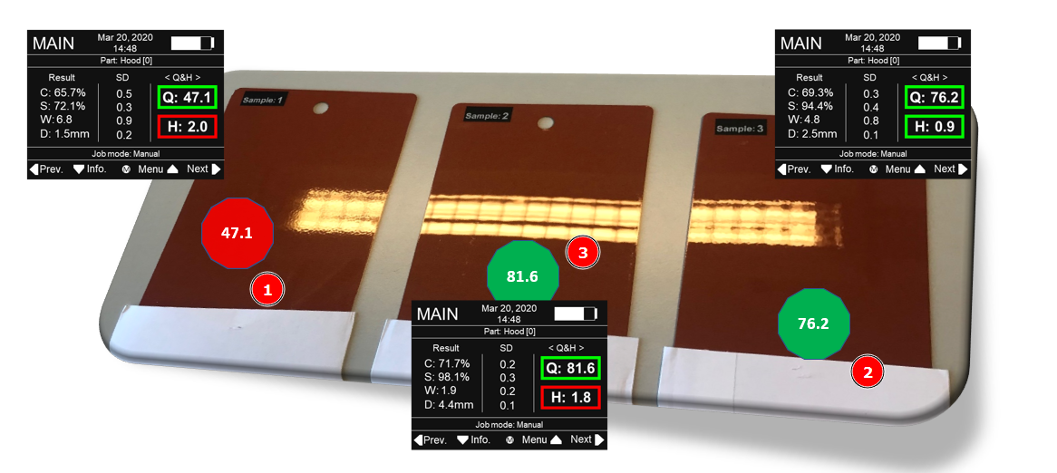
Three panels with medium (1)., good (2) and exceptional (3) quality.
Conventional instruments that control only surface waviness or DOI often ignore the effect of colour, even though colour strongly influences how defects are perceived by the customer. For example, on a black, high-contrast car, haze and poor DOI are highly visible because they reduce the depth of finish and dramatically lower perceived quality, while on a metallic silver car the same level of DOI and haze can be almost invisible to the end user. If both vehicles are controlled using only waviness and DOI limits, this can lead to unnecessary rework and over-processing on sensitive dark colours and, at the same time, an inappropriate focus on parameters that are less relevant for some lighter colours.
Typical interpretation
High Q values indicate smooth, glossy surfaces with clean, undistorted reflections; low Q values indicate visible texture, haze or orange peel that reduce perceived quality. Target Q limits can be set for production, with tighter bands used for premium or Class A surfaces.
Applications
Quality (Q) in high gloss mode is used wherever consistent visual appearance of coated surfaces is critical. Typical applications include:
- Automotive exterior body panels, bumpers, mirrors and add-on parts for meeting OEM appearance specifications and harmony targets across the vehicle.
- High gloss coatings on consumer electronics, appliances and furniture to differentiate premium finishes and control variation between batches or suppliers.
- Process development and troubleshooting for paint, clear-coat and polishing operations, where Q trends support optimisation of application, curing and sanding/buffing parameters and its colour sensitivity helps avoid over-processing or misjudging certain colours.
Harmony (TAMS High Gloss)
Harmony (H) – High gloss mode
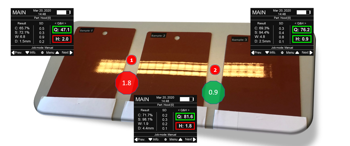
Comparing Samples 1 & 2 demonstrate poor harmony H=1.8 (1), Samles 2 & 3 show acceptable harmony H=0.9 (2)
Definition
Harmony (H) is a perception‑based index that quantifies how similar the surface texture of two high gloss painted parts appears when viewed side by side (for example fender/door or quarter panel/fuel flap). It expresses whether differences in orange peel and texture between parts are small enough to be acceptable to most observers.
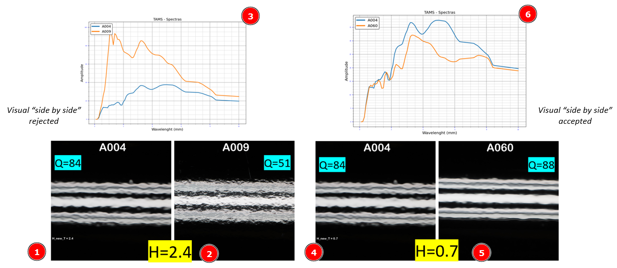
Panels (1) & (2) have dissimilar surface structure shown in the spectra (3) this results in a poor harmony H=2.4. Panels (4) and (5) have acceptable harmony H=0.7 and similar surface texture (6).
Unit and range
Harmony is a dimensionless index on the TAMS display, typically ranging from around 0.0 to 8.0 Lower values indicate good harmony (small perceived difference), while higher values indicate larger differences that are more likely to be seen as a mismatch. In practice, values below 1 are usually acceptable, whereas values clearly above 1 flag parts that may need process adjustment or rework.
Measurement conditions
Harmony is available in High Gloss Mode when the surface type is set to C‑Coat and the CC‑TAMS‑STD algorithm is selected. Harmony is calculated by comparing measurements from a reference surface (for example a master panel or agreed “good” part) to measurements from production parts, with each batch based on several readings per part to ensure stable averages.
Spectral Matching Score (SMS) – new Harmony basis
Harmony is now calculated using the Spectral Matching Score (SMS) method, which uses the complete surface texture spectrum from both surfaces being compared. Instead of relying only on differences in waviness and a single dominant texture size, the updated algorithm derives several spectral parameters from each surface, scales and weights them, and then combines them into the Harmony value. This spectral approach improves correlation with visual assessments and keeps the familiar Harmony (Hz) scale for users.
Role of waviness, dimension and sharpness
In the updated Harmony algorithm, the SMS method replaces the direct use of the Dimension (D) value in the calculation, but D is still shown on the TAMS display as a useful indicator when multiple dominant structure sizes are present. Because the full spectrum is used, sharpness‑related information from very short wavelengths is now included alongside waviness‑related components, so Harmony responds more closely to the texture features that observers actually see. Users should treat Harmony (H) as the primary acceptability index for panel‑to‑panel matching, while using D as a diagnostic aid rather than a direct quality criterion.
Typical interpretation
- H < 1.0: Panels are visually well matched in texture; differences are generally acceptable in production and in the showroom.
- H ≈ 1.0–2.0: Noticeable but often tolerable differences, which may still require attention on dark or premium Class A surfaces.
- H > 2.0: Clear texture mismatch; likely to draw attention and reduce perceived vehicle quality, typically prompting process optimisation or rework.
Sharpness (TAMS High Gloss)
Sharpness (S) – High gloss mode
Definition
Sharpness (S) is a perception‑based index that quantifies how accurately images are reflected in a high gloss surface. It describes how crisp or blurred the reflected pattern appears, linking directly to visual impressions of haze and clarity.
Unit and range
Sharpness is expressed in percent (%), from 0% (very low sharpness, heavily blurred reflection) to 100% (perfect image reproduction with no visible blur). On real automotive clear‑coat surfaces, values typically sit between these extremes depending on coating system and process settings.
Measurement conditions
Sharpness is available in High Gloss Mode when the surface type is set to C‑Coat and a high‑gloss algorithm such as CC‑TAMS‑STD is selected. Measurements should be taken on clean, defect‑free areas with good contact between the TAMS measuring base and the surface.
Meaning at different viewing distances
Sharpness characterises the surface across two practical viewing conditions:
- At close distance (approximately <0.5 m), Sharpness indicates how well the surface reproduces fine details of the reflected pattern, such as edges and small features.
- At showroom viewing distance (around 1.5 m), Sharpness is closely related to haze and clarity, describing how much the reflected image appears “milky” or washed out versus clean and transparent.
High Sharpness means that reflections remain well defined at both distances; low Sharpness indicates that fine detail is lost and the surface appears hazy or smeared.
Relationship to other parameters and indices
Sharpness works together with other TAMS parameters to describe overall appearance:
- With Contrast (C), it defines how vivid and detailed the reflection looks, especially on dark, high‑contrast colours.
- With Waviness (W) and Dimension (D), it helps separate blur caused by haze (sharpness‑related) from distortion caused by large‑scale texture or orange peel.
- A rescaled internal metric, Sharpness‑Q (Sq), uses Sharpness and Contrast as inputs to improve the perceptual weighting in the Quality (Q) index; Sq itself is not shown on the instrument but is used in the Quality calculation.
Typical interpretation
- S > 80%: Very crisp reflections with minimal haze, typical of high‑end clear‑coat finishes and well‑polished surfaces.
- S ≈ 50–80%: Poor sharpness for many production finishes.
- S < 50%: Obvious haze and loss of detail in reflections; surfaces often appear “soft” or dull, signalling coating, curing or polishing issues that reduce perceived quality.
In practice, Sharpness can be trended alongside Quality (Q) and Waviness (W) to diagnose whether loss of appearance quality is driven mainly by haze/clarity (low S) or by texture/orange peel (high W), guiding targeted adjustments to paint application, curing or polishing processes.
Waviness (TAMS High Gloss)
Waviness (W) – High gloss mode
Definition
Waviness (W) is a perception‑based index that describes the overall wavy or non‑flat character of a high gloss surface. It quantifies how strongly the reflected image is distorted by large‑scale surface waves and orange peel when viewed at typical showroom distance.
Unit and range
Waviness is reported in W‑units on a scale from 0 to 30.
- 0 W indicates a visually flat surface with almost no distortion in the reflection.
- 30 W represents a very wavy surface with strong, clearly visible distortion.
In normal automotive clear‑coat applications, most values fall between these extremes, depending on substrate, coating system and process conditions.
Measurement conditions
Waviness is available in High Gloss Mode when the surface type is set to C‑Coat and a high‑gloss algorithm such as CC‑TAMS‑STD is selected. Measurements should be made on clean, defect‑free areas with good contact between the TAMS measurement base and the surface to ensure that the full texture is captured correctly.
Visual meaning at showroom distance
Waviness is defined with respect to how an observer sees the car at around 1.5 m viewing distance. At this distance, it describes:
- The strength of the “orange peel” effect – how much straight lines and reflected features appear to ripple across the panel.
- The overall smoothness of the body shape – whether the finish looks “liquid and calm” or “wavy and restless”.
Low W gives calm, mirror‑like reflections; high W makes reflections appear broken, wavy and visually busy.
Relationship to other TAMS parameters and indices
Waviness works together with other TAMS metrics to describe appearance:
- With Sharpness (S) it helps distinguish blur due to haze (low S) from distortion due to surface texture (high W).
- With Dimension (D) it helps identify whether the dominant orange peel structure is fine or coarse.
- W is a key input to the Quality (Q) index in High Gloss Mode and is also used (via spectral methods) in the Harmony (H) index for panel‑to‑panel matching.
Typical interpretation
- W < 5: Very smooth surface with minimal visible orange peel; reflections appear calm and undistorted, suitable for premium Class A areas.
- W ≈ 5–10: Moderate orange peel that will show visible differences between processes or panels when compared directly.
- W > 10+: Strong orange peel and distortion; surface looks visibly textured and may not meet high‑end appearance requirements, often indicating the need to optimise coating, levelling or polishing steps.
By trending W alongside Quality (Q), Harmony (H), Sharpness (S) and Dimension (D), users can quickly see when loss of appearance is driven mainly by large‑scale texture and target process changes at the most influential paint stages.
Contrast (TAMS High Gloss)
Contrast (C) – High gloss mode
Definition
Contrast (C) is a colour‑dependent index that quantifies the difference between bright highlights and dark areas in the reflected image on a high gloss surface. It describes how “strong” the reflection appears and captures the influence of basecoat colour on perceived appearance.
Unit and range
Contrast is expressed in percent (%):
- White and light metallic surfaces show low contrast (<30%)).
- Deep black can approach 100% contrast.
Measurement conditions
Contrast is available in High Gloss Mode when the surface type is set to C‑Coat and a high‑gloss algorithm such as CC‑TAMS‑STD is selected. It is calculated from the reflected pattern images captured by TAMS.
Colour dependence and visual meaning
Contrast is directly linked to the colour and optical density of the surface:
- On dark, high‑contrast colours (for example black), reflections exhibit a large intensity range between bright and dark regions, so texture, haze and DOI defects are much more visible.
- On light or metallic colours with low contrast, the same physical orange peel or haze can be far less noticeable to the observer.
Because of this, Contrast acts as a bridge between colour and texture. It explains why strict texture limits that are appropriate for black cars may be unnecessarily tight for silver, and why controlling only colour‑blind metrics (such as waviness or DOI alone).
Relationship to other TAMS parameters and indices
Contrast plays a central role in the perception‑based metrics used in High Gloss Mode:
- With Sharpness (S), it defines how vivid and detailed the reflection looks – high C and high S give deep, crisp images, while low C or low S make the surface appear flat or hazy.
- It influences the Quality (Q) index, helping Q respond correctly to differences between dark and light colours by reflecting the real visual impact on the customer.
- Through its colour dependence, it supports more realistic Harmony (H) assessments across different colours, ensuring that panel‑to‑panel matching is judged in a way that aligns with human perception.
Typical interpretation
- C > 70%: High‑impact, deep colour (e.g. solid black or dark shades). Texture, orange peel and haze are very visible; tight control of Sharpness, Waviness and Harmony is usually required.
- C ≈ 30–70%: Medium contrast colours (mid‑tones, some saturated colours). Texture and haze are visible but less critical than on deep black.
- C < 30%: Low‑contrast finishes (whites, light metallics, pastel shades). The same texture level that is unacceptable on black may be visually acceptable here.
Dimension (TAMS High Gloss)
Dimension (D) – High gloss mode
Definition
Dimension (D), also referred to as Dominant Structure Size, indicates the main texture scale that an observer perceives on a high gloss surface at typical showroom viewing distance (around 1.5 m). It describes whether the orange peel structure appears fine and tight or coarse and large‑scale.
Unit and range
Dimension is expressed in millimetres (mm). Typical values for automotive clear‑coat lie between about 0.5 mm and 8 mm.
- Lower D values correspond to fine, closely spaced orangepeel.
- Higher D values correspond to coarser, more widely spaced structure.
Measurement conditions
Dimension is available in High Gloss Mode when the surface type is set to C‑Coat and a high‑gloss algorithm such as CC‑TAMS‑STD is selected. It is derived from the measured surface texture spectrum used for waviness and other appearance parameters, so it does not require any extra measurement steps beyond a normal clear‑coat reading on a clean, defect‑free area.
Visual meaning at showroom distance
At around 1.5 m, Dimension describes the characteristic spacing of the surface waves that form the orange peel pattern:
- Small D (fine structure): The surface shows a tight, fine orange peel.
- Large D (coarse structure): The surface shows broad, large‑scale waves.
Because it reflects the dominant spatial scale rather than just the amplitude, Dimension helps explain why two panels with similar waviness can still look different to the eye.
Relationship to other TAMS parameters and indices
Dimension works alongside the other High Gloss parameters:
- With Waviness (W) it separates “how strong” the orange peel is (W) from “how large” the texture cells are (D).
- It supports interpretation of Harmony (H) by indicating whether a panel‑to‑panel mismatch is mainly due to differences in texture scale. In the latest SMS‑based Harmony algorithm, D is retained as a diagnostic value even though it is no longer used directly in the H calculation.
- Together with Sharpness (S) and Contrast (C), it helps engineers understand whether perceived appearance issues are dominated by coarse body‑shape variations, finer orange peel, or haze.
Typical interpretation
- D < 1 mm: Very fine texture.
- D ≈ 1–4 mm: Shortwave orangepeel dominant in the painted surface.
- D > 4 mm: Longerwave orangepeel dominates the surface.
Bloom R ,G, B,
Surface bloom is a near‑specular scattering effect that appears as a loss of reflective contrast in a mirror‑like surface and can include a subtle colour shift that is not detected by conventional monochromatic haze meters. Standard haze meters use a light source and detector combination filtered to the photopic V(λ) response of the human eye, producing a single luminance‑weighted signal, so wavelength‑dependent scattering can be visually apparent yet remain largely undetected in the measured haze value.
To detect this phenomenon, the Aesthtix instrument uses an unfiltered white LED arranged as a 10‑degree spotlight and an RGB camera, analysing the near‑specular region of the reflected image. The bloom is quantified independently in each colour channel as a normalised ratio of the bloom signal to a calibrated specular reference signal, and the spatial extent of the bloom in each channel is reported as an area in (\text{mm}^2). The red, green and blue bloom indices are defined as:
[
B_{R} = \frac{S_{\text{bloom},R}}{S_{\text{spec},R}}
]
[
B_{G} = \frac{S_{\text{bloom},G}}{S_{\text{spec},G}}
]
[
B_{B} = \frac{S_{\text{bloom},B}}{S_{\text{spec},B}}
]
where (B_{R}, B_{G}, B_{B}) are the dimensionless bloom values for the red, green and blue channels, (S_{\text{bloom},R/G/B}) are the measured near‑specular bloom signals, and (S_{\text{spec},R/G/B}) are the corresponding calibrated specular signals used for normalisation. For each channel, the bloom size (area of the near‑specular scattering region exceeding a defined threshold) is calculated in (\text{mm}^2), providing both an intensity‑based metric ((B_{R/G/B})) and a geometric metric (bloom area) to characterise the magnitude and chromatic character of surface bloom.